Pricing Execution Rights when Rewards are Mean Reverting

[Christoph]

TL;DR: I argue that block rewards are mean reverting and derive the fair value of future proposal rights and of execution tickets assuming mean reversion. If mean-reversion is non-instantaneous, execution rights and execution tickets are valued at a premium in high MEV times and the effect is more pronounced, the fewer execution tickets are circulating, resp. the closer in time an execution right is sold to the slot for which it is valid. The forward curves for execution rights and tickets are predicted to be monotone and the forward curve is less steep the more tickets are circulating.

Appreciations to @elainehu, @tesa, Barnabé and Akaki for comments and shared insights.

Theoretical argument for mean reversion

Suppose we want to price execution rights in the future and believe that, at least in the short run, the fluctuation in value of execution rights is driven by price volatility in the crypto market. For example, it has been argued that a lot of block rewards are driven by CEX-DEX arbitrage which tend to be higher in times of high price volatility. More specifically, let’s assume the relevant volatility that drives the rewards is that of a price process (e.g. the ETH/USDC exchange rate) that can be modeled by a Geometric Brownian motion

\frac{dP_t}{P_t}=\mu dt+\sigma_tdW_t^P

where W_t^P is a standard Brownian motion and \sigma_t is the (time dependent) volatility of the price process.

The value extractable from CEX-DEX arbitrage seems to be modeled well by the concept of Loss versus Rebalancing (LVR). As argued in the LVR paper the instantaneous loss versus rebalancing in a diffusion model, such as the one above, scales proportionally with the variance of the exchange rate (see Theorem 1). If a constant fraction of LVR is captured by the validator and these arbitrage gains dominate the total block rewards, then we should expect rewards, from here on denoted by R_t, to scale proportionally with variance:

R_t\sim\sigma_t^2.

Let’s use a stochastic volatility model for modeling the exchange rate volatility. According to the Heston model of price volatility, the volatility \sigma_t follows an Ornstein-Uhlenbeck process,

d\sigma_t=-\theta\sigma_tdt+\delta dW_t^\sigma,

where W_t^{\sigma} is a another standard Brownian motion independent of W_t^P and \delta>0 is a constant.

Assuming that rewards scale proportionally with variance, as we have argued above, and applying Itô’s lemma, we find that the rewards are distributed according to a CIR process:

dR_t=\kappa(\bar{R}-R_t)dt+\xi \sqrt{R}_tdW_t^{\sigma}

where \kappa is the rate of mean reversion of rewards (volatility is mean reverting), \bar{R} are long run average rewards (which are proportional to the long run average variance) and \xi is the volatility of rewards (so the volatility of volatility). The parameters should satisfy the Feller condition 2\kappa\bar{R}\geq \xi^2 to guarantee non-negativity.

We have obtained a mean reverting process for the rewards.

Empirical argument for mean reversion

Another way to come to the same conclusion is the empirical route. In earlier work by @elainehu , it was observed that block rewards are stationary and have autocorrelation of the following kind: block values have positive correlation with the block values in the past hour and negative correlation with the block values of two hours ago.

The results in that study were obtained for data prior to the merge. However, for more recent data (blocks 18908870 to 19146791), performing an Augmented Dickey-Fuller test confirms mean reversion (with 1% confidence level) as it did in the older pre-merge data, and it does so for different way of aggregating the data: aggregated per epoch, per hour, per day and per week (the latter for a larger time window of blocks 16308165 to 19146791). The reader would probably come to the same conclusion by just eye-balling the time series data below for per-epoch, hourly, daily and weekly block rewards:

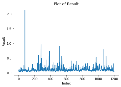
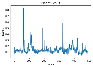
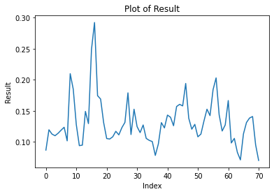
If additional evidence was needed, we can also look at fitting the data to an AR(1) model and find that the slope on the lagged rewards is between 0.1005 (per epoch) and 0.5080(per week) for all of the different ways of aggregating the data.

Deriving the fair value of execution rights

In general, let’s look at a mean reverting process

dR_t=\kappa(\bar{R}-R_t)dt+ \xi(R_t)dW_t

where \kappa is, as before, the rate of mean reversion of the process, \xi is a smooth function of rewards and W_t is a standard Brownian motion. The function \xi can be arbitrary for the purpose of fair value calculation. It matters for the distribution of rewards but not for the expected rewards. To calculate the expected rewards we can follow standard techniques (see Shreve, Stochastic Calculus for Finance II, p.152 for more details): the expectation of the Gaussian increments \mathbb{E}_0[dW_t]=0 vanishes so that we obtain a differential equation for the expectation

\mathbb{E}_0[dR_t]=\kappa(\bar{R}-\mathbb{E}_0[R_t])dt

which together with the boundary conditions \mathbb{E}_0[R_0]=R_0 and \lim_{t\to\infty}\mathbb{E}_0[R_t]=\bar{R} has the following solution:

The expectation at time 0 of rewards from execution rights at time t as a function of present rewards R_0 and long run average rewards is

\mathbb{E}_0[R_t]=e^{-\kappa t}R_0+\bar{R}(1-e^{-\kappa t}).

The fair value is obtained by discounting. If r is the discount rate, then the fair value at time 0 of the execution right for time t is

e^{-rt}(e^{-\kappa t}R_0+\bar{R}(1-e^{-\kappa t})).

Deriving the fair value of execution tickets

Execution tickets give a (probability) weighted average of different rewards in the future instead of just the rewards at a single point in time. To calculate the fair value of an execution ticket we therefore need to modify the formula above.

Let’s stick to the plain vanilla version of execution tickets, where the number of circulating tickets is held constant - each time a slot is assigned and one ticket leaves circulation a new ticket is issued (if we have a variable numbers of tickets, entry dynamics matter as well, more on that soon™). Suppose the number of circulating tickets is Q, the block time is \tau. Thus, the fraction of tickets that were issued at time 0 or before and are still in circulation at time t decays exponentially (if you wonder why that is you might want think of the metaphor of a continuously stirred tank)

Qe^{-\frac{t}{Q\tau}}.

This formula is of course a continuous approximation of the discrete reality. Differentiating it with respect to t, gives us weights \tfrac{1}{\tau}e^{-\frac{t}{Q\tau}} to calculate the weighted average of rewards that correspond to the expected total value of the Q tickets in circulation at time 0,

\mathbb{E}_0\int_0^\infty \tfrac{1}{\tau}e^{-(r+1/(Q\tau))t}R_tdt=\int_0^\infty \tfrac{1}{\tau}e^{-(r+1/(Q\tau))t}\left(e^{-\kappa t}R_0+\bar{R}(1-e^{-\kappa t})\right) dt\\=\frac{1}{\tau}\left(\frac{R_0-\bar{R}}{r+1/(Q\tau)+\kappa}+\frac{\bar{R}}{r+1/(Q\tau)}\right)

Since execution tickets are fungible the fair value of an execution ticket is obtained by dividing the previous expression by the number of tickets:

\frac{1}{Q\tau}\left(\frac{R_0-\bar{R}}{r+1/(Q\tau)+\kappa}+\frac{\bar{R}}{r+1/(Q\tau)}\right)=\frac{R_0-\bar{R}}{1+(r+\kappa)Q\tau}+\frac{\bar{R}}{1+rQ\tau}.

To summarize:

The fair value of an execution ticket for a circulating supply of Q tickets is

\frac{R_0-\bar{R}}{1+(r+\kappa)Q\tau}+\frac{\bar{R}}{1+rQ\tau}.

Note the difference between this formula and the formula for valuing execution tickets with constant expected rewards as analyzed here: the latter is obtained as limit as \kappa\to\infty, so that rewards only depend on the average rewards \bar{R} (\mu_R in the notation of that post) and not on the level of present rewards R_0. Thus only the second term is present, \bar{R}/(1+rQ\tau). Modulo notation (r=d and Q=n) this is exactly the expression obtained here (block time is normalized to \tau=1 in their case). Thus, the main difference is that with non-instantaneous mean reversion, the value of an execution ticket should be higher in high MEV times, and the effect is more pronounced the fewer execution tickets are circulating and hence the sooner in expectation the execution rewards accrue.

Forward prices and realized values

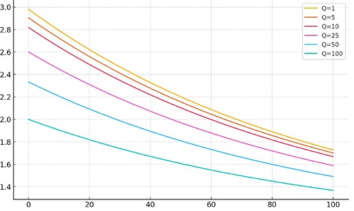
To illustrate the effect of mean-reversion we can for example look at the implied forward price of execution tickets at a mean-reversion rate of 1%. This is the present expected value of an execution ticket issued in the future. Below I have plotted the forward prices as a function of the number of blocks in the future for the case that the latest block has a value of 3ETH and the mean level of block rewards is 1ETH for different numbers of execution tickets in circulation.

These curves resemble the term structure of volatility in other asset classes, e.g. equities, where we generally observe convergence to the long-run mean for the forward curve of volatility. Execution tickets, as a weighted average of future execution rewards, are more dependent on future rewards the more tickets are circulating and therefore have a less steep forward curve the more tickets are circulating.

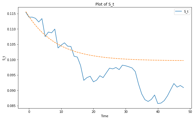
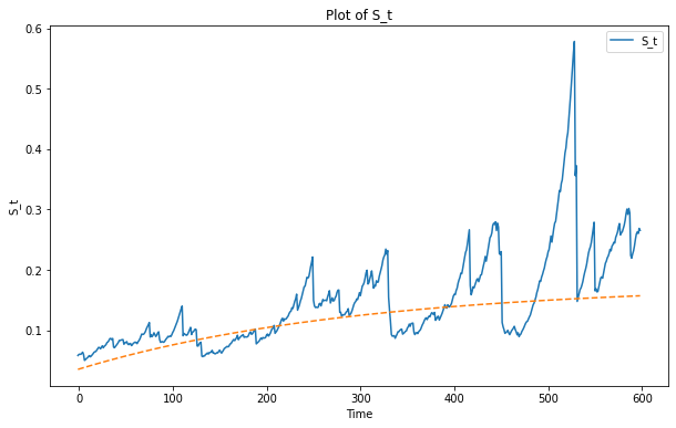
Realized rewards are of course very volatile so that the forward price might be off the realized rewards, as in the following example sample where I have calibrated the forward curve from data (see the discussion below for the parameter estimation):

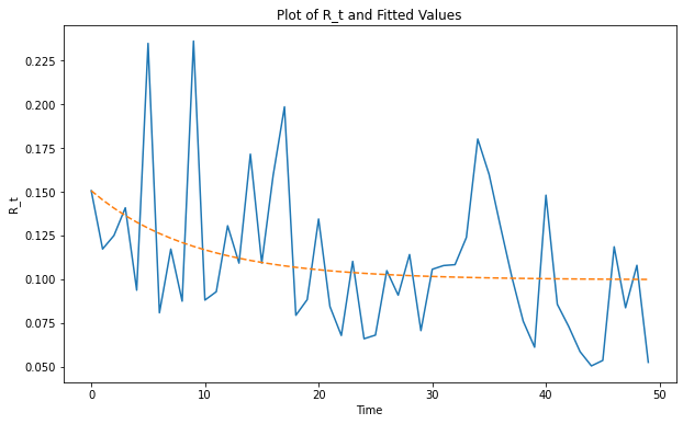
However, execution tickets have a smoothing effect on rewards. Here I plot, for the same sample, the predicted forwards prices at time 0 for execution tickets and the actually realized average profits of an execution ticket bought at different points in time.

Similarly, the forward curve is increasing if block rewards are under the long run mean, as in the

Estimating the convergence parameter

I am not a statistician, so take the following with caution, but I’m a pretty sure that the parameters \kappa and \bar{R} can be estimated with a OLS regression: Discretizing the model, we obtain the equation:

R_{t+\Delta t}-R_t=\kappa(\bar{R}-R_t)\Delta t+\xi(R_t) \sqrt{\Delta t}\epsilon_t

Let us look at the simplest case of constant variance which fits empirical data quite okay, \xi(R_t)\equiv \xi. In that case we end up with a linear regression:

R_{t+\Delta t}-R_t=\alpha+\beta R_t+\tilde{\epsilon}_t,

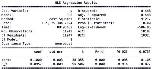
The parameter \kappa can be estimated by \hat{\kappa}=-\hat{\beta}/\Delta t and the mean level by \hat{\bar{R}}=\hat{\alpha}/(\hat{\kappa}\Delta t ) where \tilde{\epsilon}_t has mean 0 and variance \xi\sqrt{\Delta t} . I ran the regression on per-epoch aggregated data and got the following output:

Thus, we get the estimates of \hat{\kappa}=0.8957/6.4min\approx 0.14/min and \hat{\bar{R}}=0.1/(6.4*0.14)\approx0.11\,\text{ETH}.

Similarly if we would assume that the variance scales with the square root of rewards, \xi(R_t)=\sqrt{R_t}, as discussed above, then we could run the regression

y\equiv \frac{R_{t+\Delta t}-R_t}{\sqrt{R_t}}=\beta_1\frac{1}{\sqrt{R_t}}+\beta_2 \sqrt{R_t}+\tilde{\epsilon}_t\equiv \beta_1 x_{1,t}+\beta_2x_{2,t}+\tilde{\epsilon}_t,

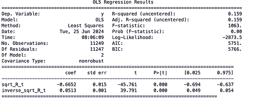
and obtain \hat{\kappa}=-\hat{\beta}_2/\Delta t and \bar{R}=\hat{\beta}_1/\hat{\kappa}. I ran a regression for this variance specifications, aggregating data again on an epoch level and got a worse fit:

However, the estimates are in the same ball park as the previous ones:

\hat{\kappa}=0.6652/6.4min\approx 0.1/min and \hat{\bar{R}}=0.0513/(6.4*0.1)\approx0.08\,\text{ETH}.

We can summarize the result as follows:

The empirically observed speed of mean-reversion is \sim 2\% per slot.

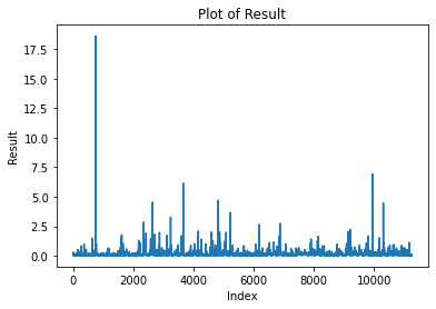
There are some caveats to mention here: with the short time window of an epoch (32 slots) there is a lot of noise picked up and averaging over larger time windows might give a more accurate estimation. Residuals are slightly heavy-tailed, suggesting that normality is violated. In general, the 2% seems to over-estimate the per-slot mean-reversion rate, and I get lower rates for hourly averaged data. Further backtesting and estimation would be necessary to get a more accurate estimate.

Extending the model to include a drift

While short run rewards data is stationary, we might expect that in the long run rewards are increasing if we believe that the Ethereum blockchain attract more and more valuable usage. It is easy to adapt our model by letting average returns grow over time:

dR_t=\kappa(\bar{R}_t-R_t)dt+ \xi(R_t)dW_t^{\nu}\\ d\bar{R}_t=\mu\bar{R}_tdt

Thus, we have \bar{R}_t=e^{\mu t} for a drift paramater \mu\geq0. A similar calculation as before yields:

\mathbb{E}_0[R_t]=e^{-\kappa t}R_0+\frac{\kappa\bar{R}_t}{\mu+\kappa}(1-e^{-\kappa t}).

Accordingly, the value of an execution ticket is

\frac{R_0}{1+(r+\kappa)Q\tau}+\frac{\kappa}{\mu+\kappa}\left(\frac{\bar{R}_0}{1+(r-\mu)Q\tau}-\frac{\bar{R}_0}{1+(r-\mu+\kappa)Q\tau}\right).