Modelling Realised Extractable Value in Proof of Stake Ethereum - an update of validator return post-merge
The Ethereum proof of work (PoW) mining ended on September 15, 2022. The transition to proof of stake (PoS) changes the current static block reward on the execution layer to an algorithmic reward on the consensus layer in the beacon chain protocol. Although the maximal extractable value (MEV) will not be directly affected by the merge, the annual validator return which consists of both the block reward and the MEV will change.
In this paper, a dynamic approach is proposed to model the MEV using the on chain historical observable data - the realised extractable value (REV). Combining the modelled REV with the simulated block reward post-merge, the model is able to estimate a range of validator returns under different network conditions given a fixed number of validators.
The unique insight this paper provides, when compared to similar validator return analysis in the existing space, lies in:
- the migration from a fixed average or median MEV to a dynamically modelled MEV;
- the consideration of exogenous variables i.e. gas price, base fee, Ethereum price etc. and their potential effects on MEV;
- the usage of empirical data (REV) to model the correlations between the exogenous variables and MEV;
- the construction of time-dependencies in modelling REV, i.e. using the recent past to predict the near future;
- the inclusion of confidence intervals in each point-in-time REV prediction;
- the replacement of a fixed validator return with a dynamic range of returns that are responsive to different network conditions given a specific number of validators.
The main findings from this study on REV can be summarised as below:
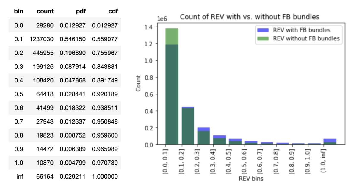
- 80% of the blocks have an REV (or block net profit) <= 0.25 ETH; 90% <= 0.45 ETH and 99% <= 2ETH.
- REV seems to be higher during UTC hour 13:00 to 20:00 when looking at hourly frequency through aggregation by median.
- REV in the past hour (t-1) has a positive correlation with the current hour; whereas REV in the hour before the last hour (t-2) has a negative correlation.
- Gas price and gas units used have a positive correlation with REV while base fee has a negative correlation.
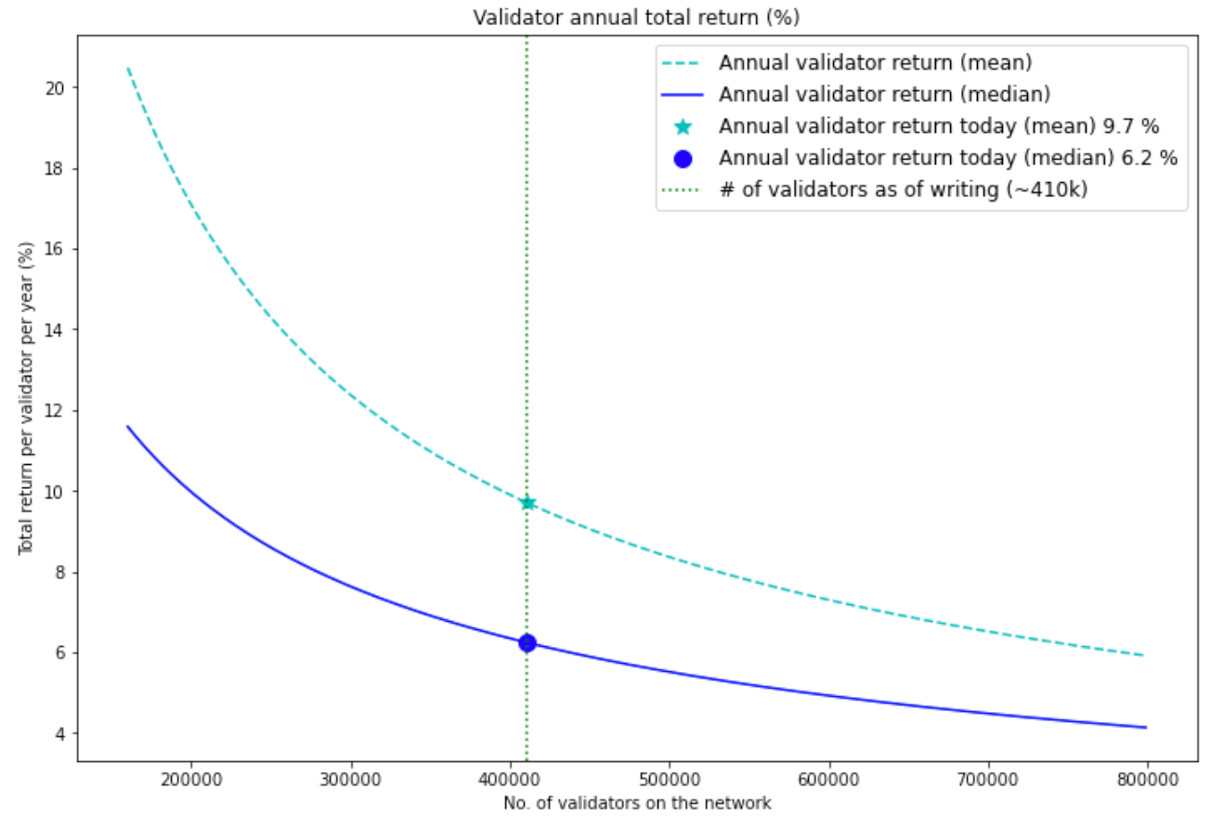
- Validators can expect a return ranging from 4.79% to 7.8% under different network conditions given 410,499 validators on the network.
The data used in this paper is provided by Taarush Vemulapalli at Flashbots. Full analysis and code are available here.
Introduction
Flashbots have published the analysis of MEV in eth2 - an early exploration_{[1]} last summer. In this analysis, the annual validator return is estimated by the median block net profit along with the simulated consensus layer block reward post-merge.
The chart below compares the two fixed value methods that are often used by other analysis to estimate the annual validator return - mean and median. At today’s level of number of validators (~410k), the difference between the two methods is 3.5%, which is quite a difference and could be confusing.
The main problem with this approach is the constant median (or mean) block net profit assumed in the estimation. In practice, profits from each block is very different and can be affected by many factors such as gas price and base fee. Although median is a more robust method to handle outliers with extremely high values, it is still a rough estimation with only one fixed number.
REV can be affected by the ever changing conditions of the Ethereum network, therefore factors such as gas price, base fee, Ethereum’s price etc. should be taken into consideration when estimating the validator return.
MEV vs. REV
The maximal extractible value - MEV is a theoretical concept that defines how much ETH a miner can extract given a set of user transactions, initial state and contract. However, in practice there is always a portion of the extractable value that is unobservable on chain. For example, if a searcher pays the miner through L2 network or through bank transfers, the profit extracted by the miner through these methods will not be observable.
Therefore, the concept of realised extractable value (REV) is defined to distinguish the portion of extractable value that can be observed through data on chain from the theoretical MEV. REV is the actual value extracted from the blockchain from MEV opportunities. For more details about defining and quantifying REV, refer to the paper Quantifying Realised Extractable Value_{[2]} .

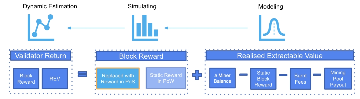
In order to estimate MEV, we have to accept the fact that REV is always less than MEV and the best we can do is to collect the observable extractable value REV. REV, also referred to as block net profit in previous sections, is calculated as the miner balance change before and after mining a block, filtered to remove any static block reward from proof of work and any transactions originated from the validator’s address such as mining pool payout.
As @pintail pointed out, the value extracted from the blockchain doesn’t all go to the validator; some of them are captured by searchers and other intermediaries. Therefore, it is worth pointing out that the REV calculation here approximate the extractable value as the validator balance difference based on the past PoW data that miners get the majority portion of the REV. Post-merge this could be different and the validity of this assumption can only be tested with longer periods of data after the merge.
Modelling REV
The block level data used in this paper is collected after the London fork from block number 12965000 to 15229999; the REV is then calculated as explained in the previous section and used along with the exogenous variables to build estimation models.
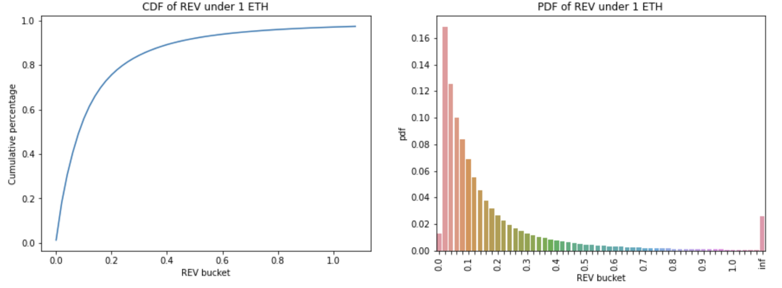
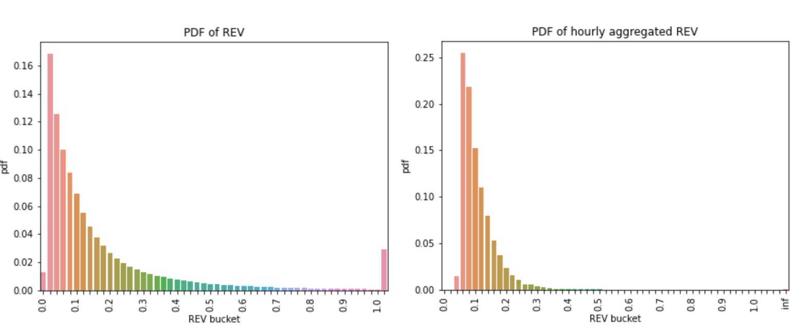
Looking at the REV cumulative distribution function (CDF) and the probability density function (PDF), 56% of the blocks have an REV of less than or equal to 0.1 ETH; 97% of them are less than or equal to 1 ETH. Most of the REV per block seems to concentrate at the lower end of the buckets.
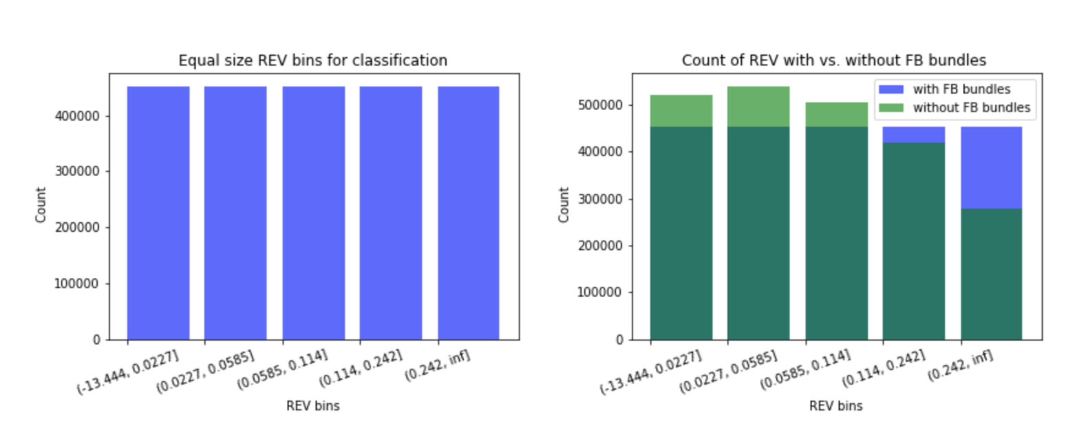
The REV per block is also categorised into blocks with Flashbots (FB) bundles and without. The green bars are REV from blocks without FB bundles whereas the purple bars are REV from blocks with FB bundles; the darker green bars are the overlapping parts. The additional block profits provided by the FB bundles in excess of the blocks without are in purple (right-hand-side chart below). It is interesting to see the advantage of using FB bundles lies in the higher REV buckets of more than 0.1 ETH; the proportion of the excess profits from FB bundles is also higher in the larger than 1 ETH bucket.
The REV data collected post the London fork has over 2 million blocks. Training such a large amount of data to build a model could be computationally expensive. Furthermore, if a time-series model is used, the time intervals in the data need to be equal, which is not the case in the PoW world where the block time is not fixed. Therefore, it makes sense to aggregate the data to an equal time interval for the purpose of not only reducing computation time but also making the data suitable for time-series models.
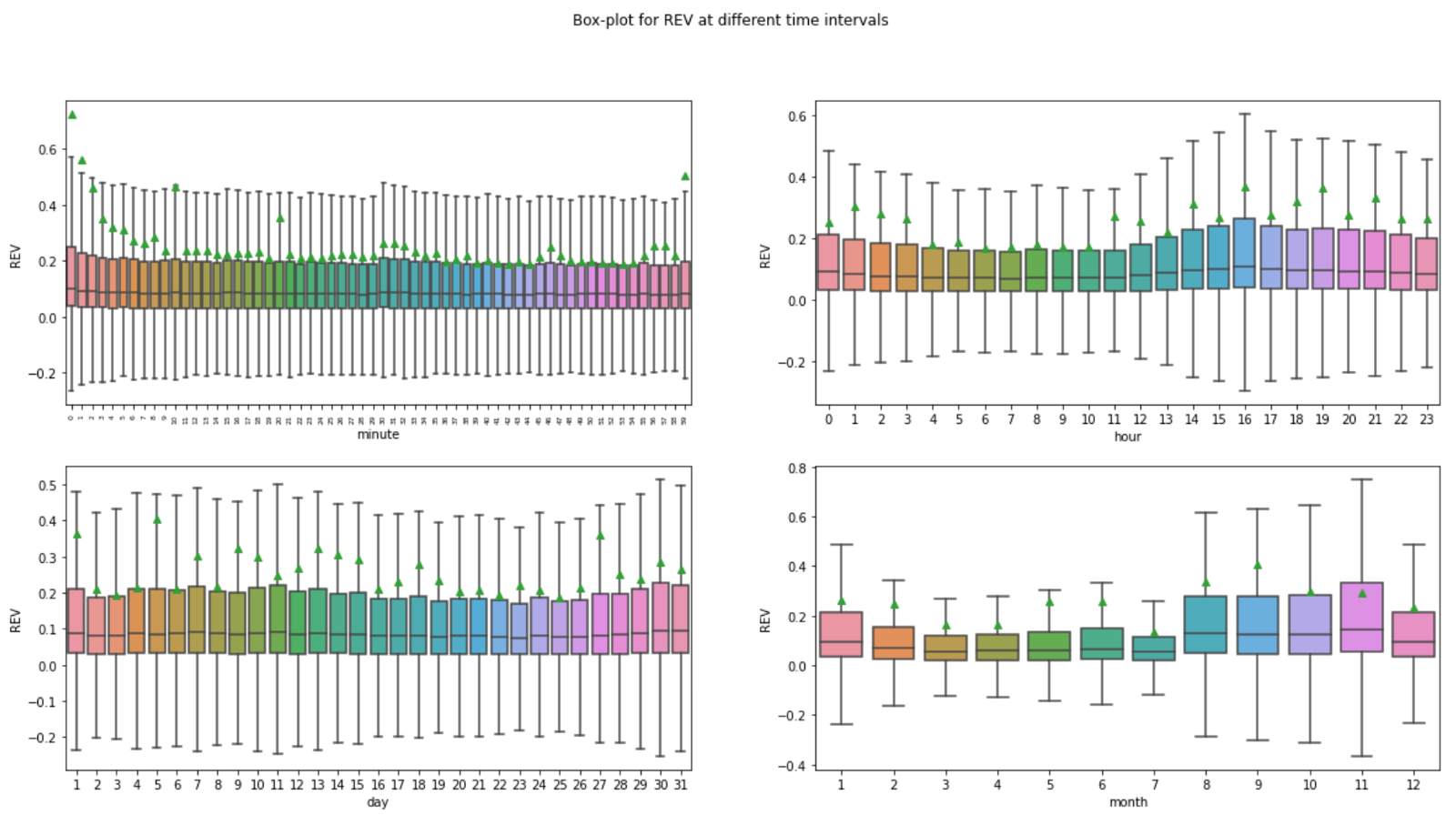
In order to decide at which frequency the block level data should be aggregated, box-plots of REVs at different time intervals are shown below to help identify potential seasonality or trend in REV data.
The box-plots’ size and median in the minute and daily charts seem relatively stable whereas the hourly and monthly chart show some variations. Although the median REVs are higher in the months from August to November in the monthly chart, the data is only collected over 1 year and the sample size might not be large enough to be representative. In the hourly chart, the median REVs are slightly higher during UTC hours 13:00 to 20:00, which coincide with the U.S. stock markets opening time.
Since the hourly data shows a degree of seasonality, the optimal choice would be to aggregate the block level data to hourly. The probability density charts below reveal another benefit of the hourly aggregated data compared to the block level data - the absence of outliers. The cluster of large REVs in the block level density chart (left) disappears once the data is aggregated to hourly (right).
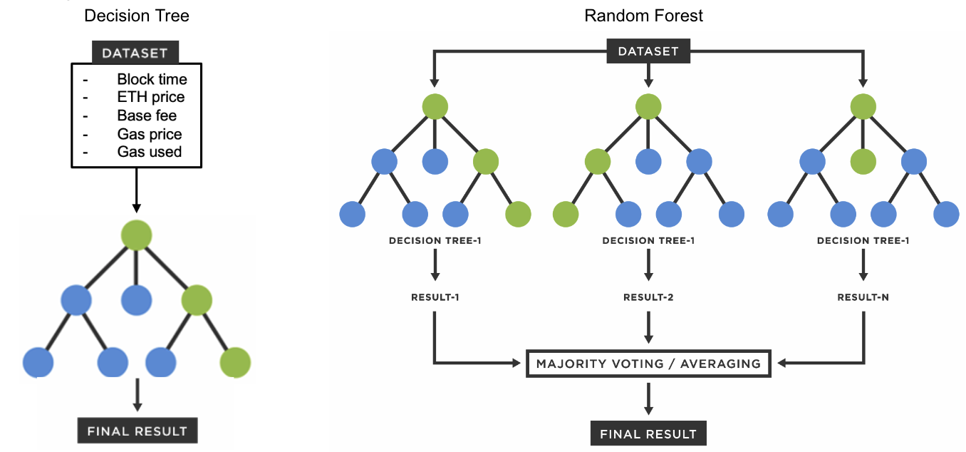
Classification and Regression Tree Method
In this section, two tree methods are used to model REV using the hourly data - decision tree classifier _{[3]} and random forest regressor _{[4]} . The former builds one tree that predicts REV as a class; whereas the latter builds multiple trees and aggregates them to predicts REV as a continuous variable.
Classification Tree
In the decision tree classification model, REV is divided into different buckets and the model will predict the probability of REV falling into one of these buckets using the five exogenous variables available in the data - gas price, gas units used, base fee, Ethereum price and block time.
The bar charts show the five equal size buckets the REVs are divided into for the classification model. The reason to create equal size buckets is to avoid the problem of predicting the most frequent class. Due to the uneven distribution of REV and the high concentration in the lower REV buckets, when the bin size is unequal, a classifier can simply predict the most frequent class and achieve a high accuracy score without any efforts. The equal size bins ensure all the classes have the same number of data points and the model has to provide enough predictive power to distinguish each class.
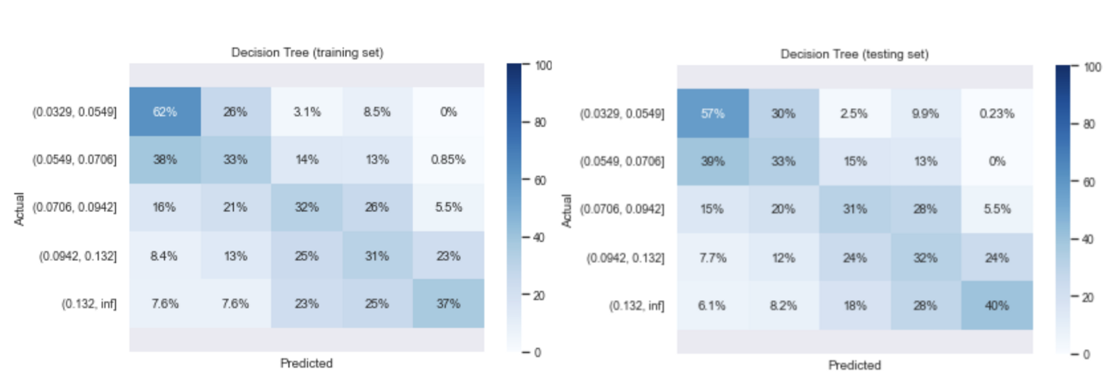
The hourly REV data is split randomly into 75% training set and 25% testing set. The initial model is trained on trials of different hyperparameters, such as the maximum tree depth, the minimum sample leaf etc. to find the optimal model. The selected optimal model is then used to predict on both the training set and the testing set to ensure the model performance from the two are similar and the training set is not overfitted.
By plotting the accuracy score with different trials of maximum tree depths for the training and testing set, the optimal point is found at 5 where the accuracy scores between the two sets start to diverge.
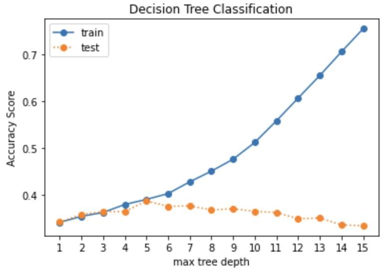
The final decision tree model is trained with a tree depth of 5, and has an accuracy score of 39% from both the training and the testing set. Although there is very little overfitting in the model as shown by the similar accuracy scores from both sets, the model performance is not very good. There are quite a lot of mis-classification in each class as shown in the confusion matrices.
Regression Tree
In the attempt to improve the model performance, a random forest regressor model is used. Random forest is similar to decision tree, except that it uses ensemble method to create sub-samples to build many decision trees and the results are aggregated through averaging. Instead of predicting a class, the model will predict a continuous REV under the random forest regressor.
Similarly, by plotting the performance metric R-squared of the training and testing set against different trials of maximum tree depth, the optimal tree depth is found at 4.

The model performance measured by R-squared from the training set is 44.4% while from the testing set it is 43.9%. The plots below show the predicted vs. the actual REV during the period of time the historical REV data is collected. 82% of the actual REV points fall into the model predicted confidence intervals [2.5%, 97.5%].
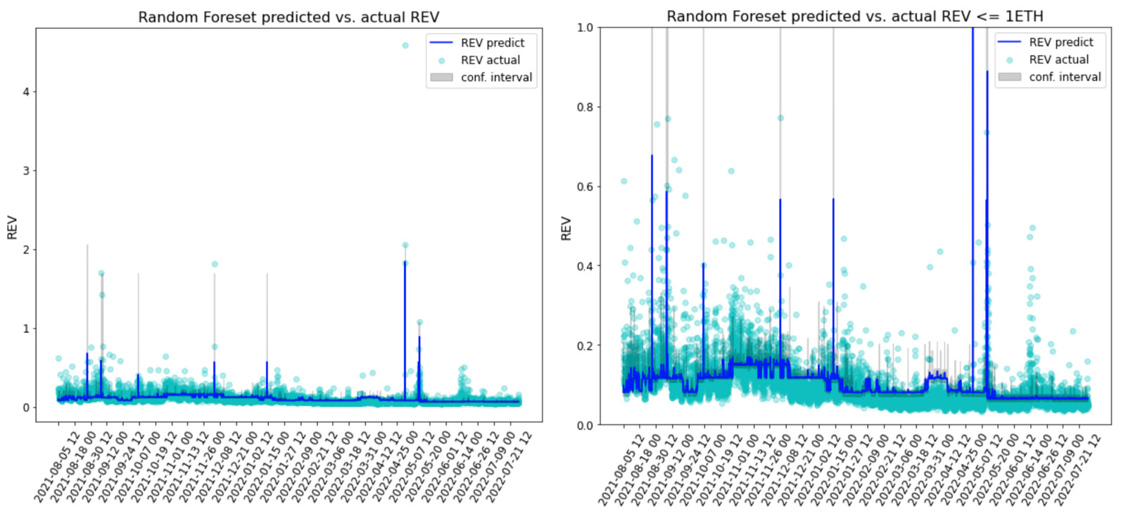
Although the performance has improved slightly compared to the decision tree classifier, there are still a fair amount of under-estimation as shown in the predicted vs. actual REV scatter plots. When zoomed in to the REVs under 1ETH, which is where most of the data points are, the predictions seem flat in the recent downturn period from May 2022.

Time-Series Model
Given the unsatisfactory performance from the previous two models which treat the hourly REVs independently, it makes sense to assess if there is any inter-temporal correlations between REVs, i.e. if the recent past REV has an effect on the current REV.
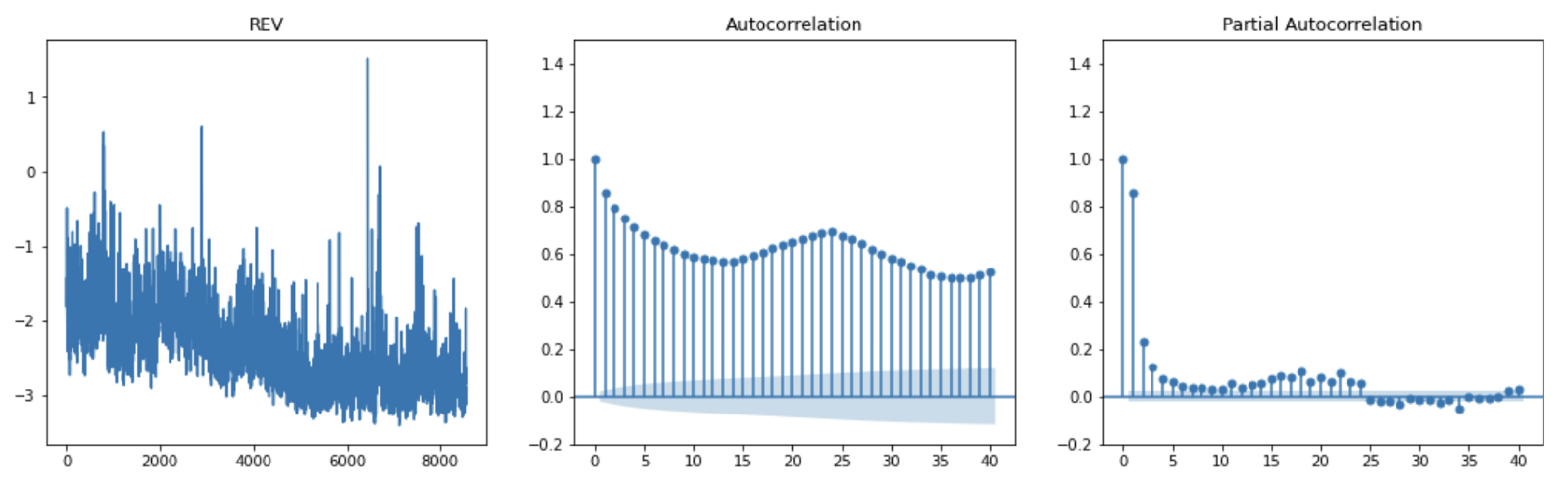
As shown in the autocorrelation and time-dependency charts below, although REV is a stationary time-series (at 1% significance level using Augmented Dickey-Fuller test), it has a positive correlation with its lag terms.

The Autoregressive Integrated Moving Average (ARIMA) model is a time-series model that allows the dependent variable’s lag(s), difference(s) and the error terms’ lag(s) to be included in a regression as independent variables. This is very useful when time dependencies exist in the data and the inter-temporal correlation of the target variable is high.
A generic ARIMA(p,d,q) process can be described as _{[5]} _{[6]} :
where X_t is the dependent variable; L is the lag operator; d is the degree of differencing; p is the number of time lags of the autoregressive terms; q is the number of lags of the moving-average terms; \delta is the drift term; \psi_i is the parameter of the $i$th lag term; \theta_i is the parameter of the moving average term and \epsilon_t is the error term.
In addition to the endogenous time-dependent factors, the five exogenous variables can also be included in the ARIMA model. The following formula describes the set up of the ARIMA model for the REV estimation:
where REV_t is the realised extractable value at time t; p and q are the total number of REV time lags and moving average lags tried in the model iterations; d is the number of differencing tried on REV_t; \alpha_i is the parameter of the $i$th time lag term; \gamma_j is the parameter of the $j$th moving average lag term; n is the total number of exogenous variables and \beta_k is the parameter of the exogenous variable V_k.
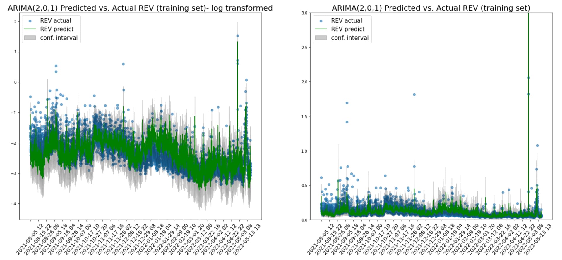
After multiple iterations of different REV time lag, moving average lag and the order differencing, the optimal model turns out to be ARIMA(2,0,1) - two REV time lags, no differencing and 1 moving average lag. The exogenous variables that turn out to be significant are - gas price, gas used and base fee.
It is interesting to see the past 1 hour REV has a positive correlation with the current hour REV whereas the hour before the past 1 hour has a negative correlation. The momentum in the high REV from the previous hour seems to carry on to the current hour; but if a high REV was observed 2 hours ago, the current hour is expected to have a lower REV.
The coefficients from the exogenous variables seem to be aligned with expectations and can be explained intuitively. An increase in the gas price and the units of gas used indicate an increasing level of traffic and demand in the network, leading to more MEV opportunities and higher amounts of extractable value. On the opposite, since base fee is deducted from the total block profit, a higher base fee will result in a lower REV (or net profit) from the block.
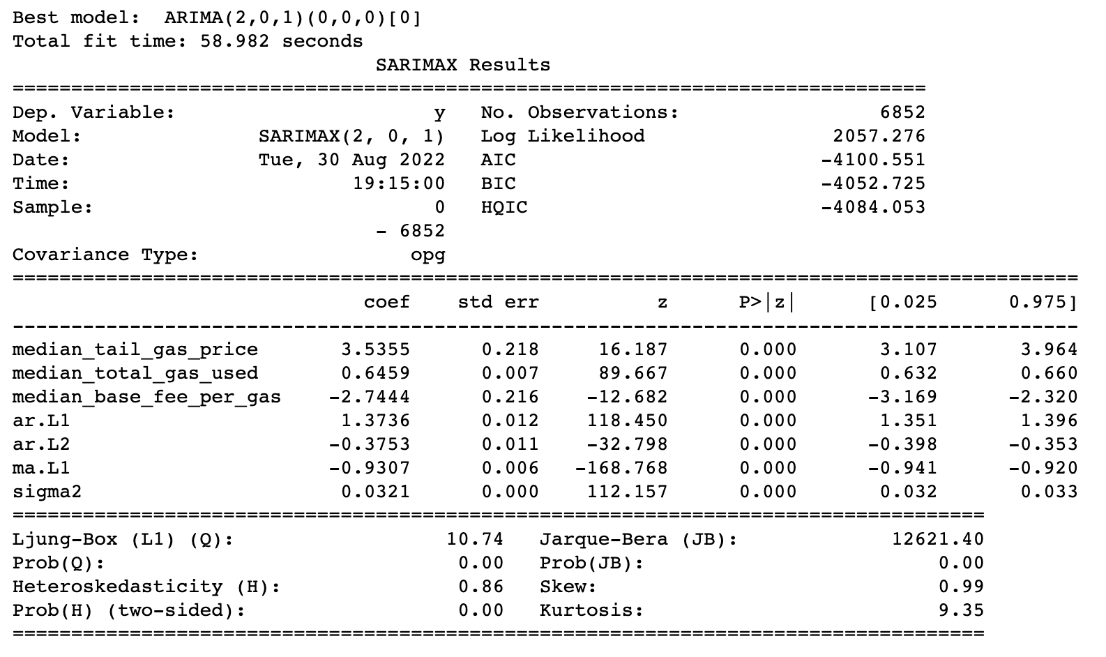
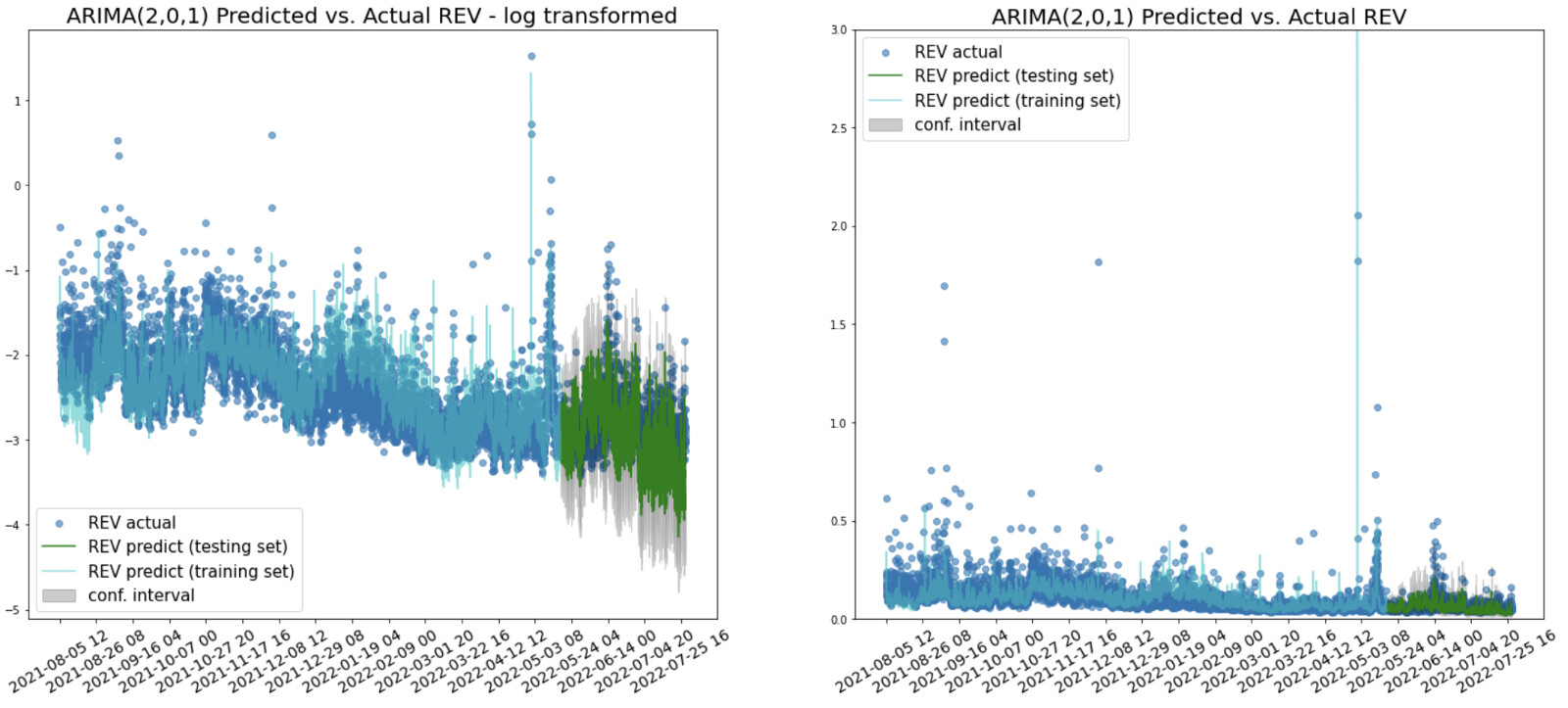
The model performance measured by the mean absolute percentage error (MAPE) is 0.12 for both the training set and testing set. The correlation coefficient between the predicted and the actual REV for the training set is 78% whereas for the testing set it is 61%.
In the training set plots, the predictions (green) and its confidence intervals (grey) are able to capture most of the extreme points and the fluctuations over time. This is a better outcome than the random forest regressor which predicts relatively flat REVs over time.
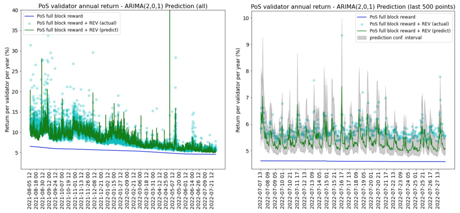
In the testing set where the recent downturn period started, the model is also able to capture the downward trend from May 2022. 91% of the actual REV points fall into the prediction’s confidence interval in the testing set.
Dynamic Validator Return
Instead of using a fixed median REV to estimate the validator return, a dynamic return based on different network conditions can be obtained using the model predicted REVs and the simulated block reward in PoS, which is dependent on multiple factors such as number of validators, penalties, participation rate etc.
The two models selected from the previous sections that are used for the REV predictions are:
Random Forest Regressor: 500 trees with 4 levels of tree depth.
ARIMA (2,0,1): Log-transformed variables with 2 lag terms, 0 differencing and 1 moving average prediction.
The validator return is estimated as the sum of the block reward from the beacon chain and the predicted REV. The return is annualised by dividing the total ETH amount by 32 ETH per validator.
The model predictions are at hourly frequency. The blue line in the charts below is the return from the full base reward in PoS; the green line is the total predicted annual return, including the full base reward and the predicted REV.
Although random forest regressor is able to capture the spikes in some high REV periods as shown in the chart on the left, during the recent periods the predictions are very flat (right). This is due to random forest’s method of averaging across all trees to get the final predictions. The past high return periods have more weights in the calibration using this method and the recent low REV periods do not show a dynamic and responsive prediction.
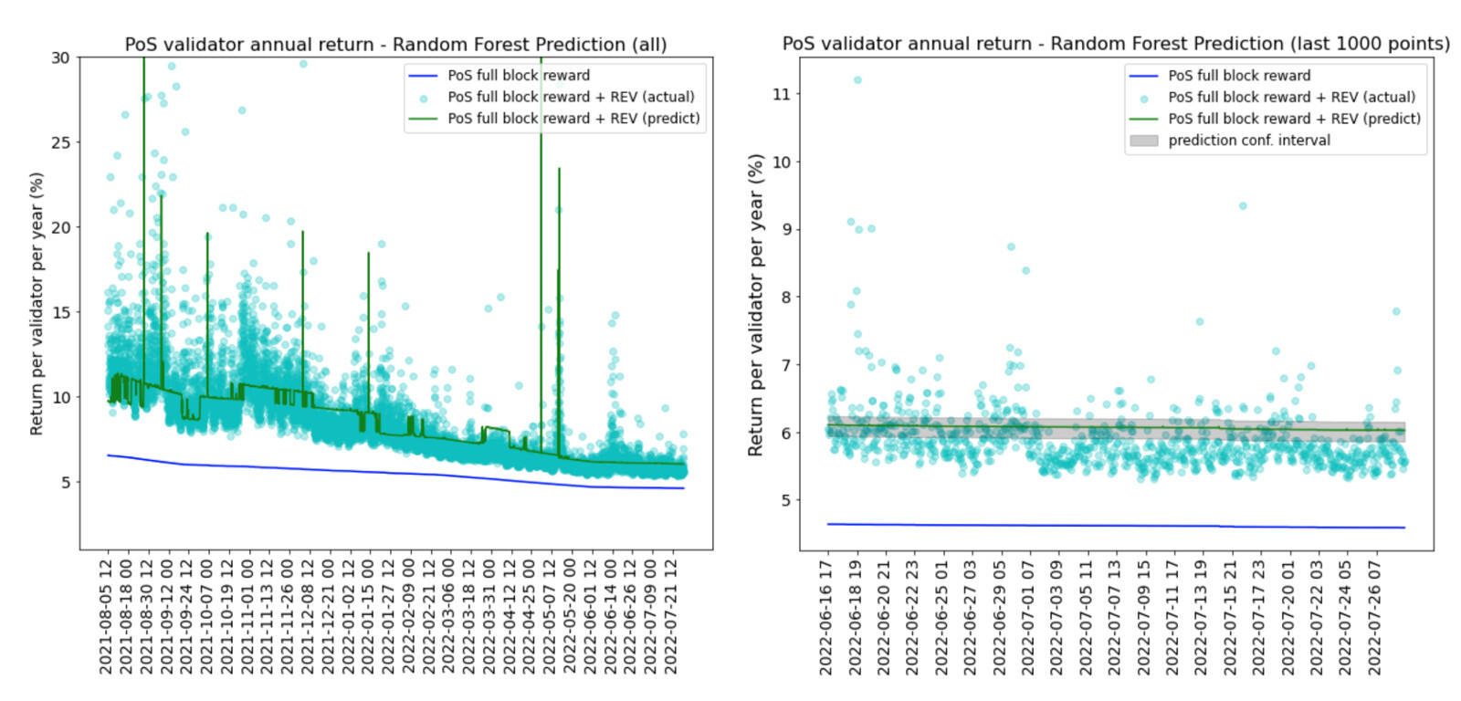
On the contrary, the ARIMA model not only captures the high REV periods in 2021 but also predicts a more responsive REV in the recent downturn periods. The confidence intervals cover a wide range of returns when REV is volatile.
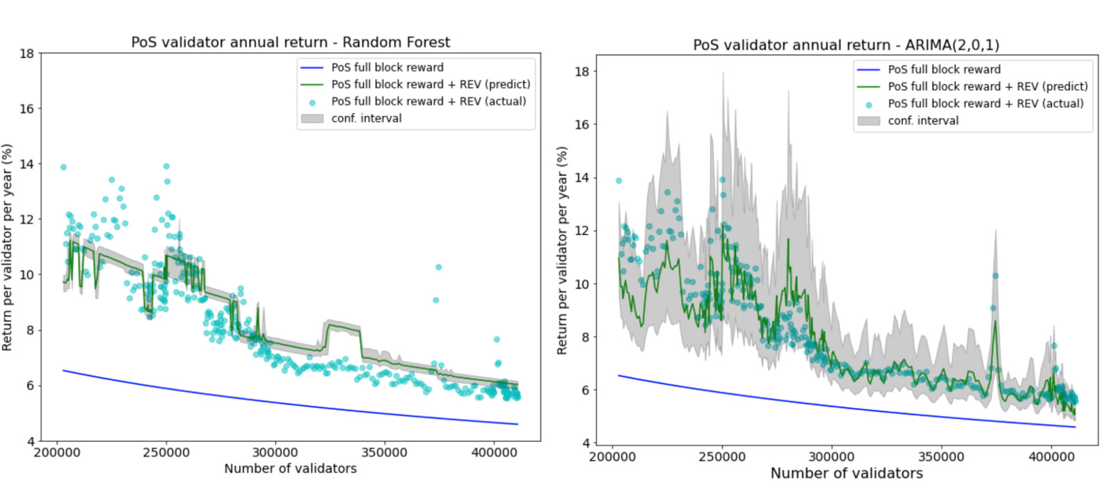
Since the REVs are predicted at an hourly frequency, to plot the annual validator return against each unique number of validators, the predictions need to be aggregated at a validator level. This is done by taking the median of the predictions from a given number of validators.
It is clear that random forest regressor’s predictions are less dynamic than the ARIMA model and the confidence intervals are too narrow to cover the actual REV points. The ARIMA model is better at handling both volatile and stable periods of REV - the confidence intervals are wider when REV is volatile and narrower when REV is more stable.
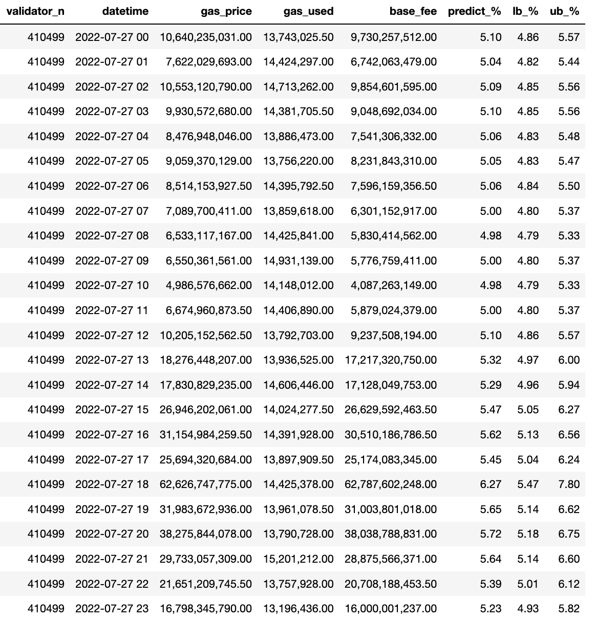
The table below shows an example of different annual validator returns and the lower bound (2.5%) and upper bound (97.5%) predicted using the ARIMA model given 410499 validators and different inputs of the gas price, gas used and base fee. Note that the actual REV from the previous hour and the hour before also contribute to the prediction but they are not shown in the table.
The best case prediction is when the gas price and gas units used more than doubled in the hour of 18:00 on 2022-07-27, reaching an upper bound prediction of 7.8% annual return. The worst case is 4.79% when the lowest gas price and gas used are observed.
Conclusion
In this paper, we explore three methodologies to model MEV using the historical observed REV data. The decision tree classifier and the random forest regressor models do not perform very well in predicting the hourly REV. The ARIMA model with REV time lags and three exogenous variables gives a better performance. The predictions are able to capture the volatility in the REV as well as the generic downward trend in the recent months since May 2022.
With the recent past REVs and the different levels of gas price, gas units used and base fee, the ARIMA model is able to predict a validator return that responds dynamically to these factors. The approach proposed in this paper therefore provides validators a new way to anticipate the profit they can make from a block in the post-merge proof of state Ethereum network.
Open Questions
The variables included in the models are only limited to those available at the time the data was collected. There are many other variables that could also have an impact on REV. It would be interesting to know:
- Does Ethereum’s price volatility or its trading volume have an impact on the hourly REV?
- Is there any other ERC-20 token that could have an impact on REV?
Since the proposed ARIMA model uses data from PoW and predicts at an hourly frequency, it is natural to ask the following questions after the merge in PoS:
- Does the 12 seconds fixed block time in PoS have any effect on the REV prediction compared to the changing block time in PoW?
- Does the ARIMA model performance improve when the model is calibrated at a higher (or lower) frequency post-merge, i.e. 12 seconds or multiples of the fixed block time?
All the validator return in this paper assumes validators get the full base reward, the network participation rate is 100% and the expected number of blocks proposed by each validator is 6 blocks (the average from a binomial distribution with 410,000 validators). However, less ideal scenarios could lead to a lower validator return:
- What happens if validators get penalised because they fail to attest the header, target or source?
- The unluckiest 1% validator only gets to propose 1 block per year. What is the annual return for the unluckiest 1 %?
- How much less return the validators get when participation rate drops?
- How would the validator return change when all the above worst case scenarios happen at the same time?
Last but not least, are there any other methodologies that can be used to predict REV? Here are some alternative modelling options:
- Neural network enhanced autoregressive model (NNAR)
- Markov Chain state transition matrix model
References
[1]: MEV in eth2 - an early exploration MEV in eth2 - an early exploration - HackMD
[2]: Quantifying Realized Extractable Value Quantifying Realized Extractable Value - HackMD
[3]: Decision tree classifier from Scikit Learn sklearn.tree.DecisionTreeClassifier — scikit-learn 1.1.2 documentation
[4]: Random forest regressor from Scikit Learn sklearn.ensemble.RandomForestRegressor — scikit-learn 1.1.2 documentation
[5]: Autoregressive integrated moving average Autoregressive integrated moving average - Wikipedia
[6]: Auto ARIMA from pmdarima: ARIMA estimators for Python pmdarima.arima.auto_arima — pmdarima 2.0.1 documentation
[7]: SBC 2022 MEV Workshop slides: Modeling Realised Extractable Value in Proof-of-stake Ethereum - Google Slides
[8] Flashbots data transparency issues 6: Validator rewards post-merge
[9] Flashbots eth2-research issue 4: Questions on the ETH2 MEV analysis update