The faint sound of a money printer - Part 4 of 5
The subject of this series is an unverified arbitrage bot on Arbitrum reconstructed here from its bytecode.
The contract carries a natural logarithm and an exponential it built by hand, in integer arithmetic (because the EVM has no floating point and no logarithm instruction) and they run only on the rare occasion it decides an opportunity is worth real money.
Earlier parts in the series cover where those two functions were dug out, the bot’s behavior and the format of its instructions, but this part should be readable without any of them.
Last part ended revealing two functions the contract had no visible use for. Nothing in the arbitrage we had described up to that point (borrow a token, swap it, swap it back, repay) needs a logarithm anywhere in it, and yet there one was, hand-built and paid for in gas by an operator who has been trying to save every unit of it since the beginning.
Here’s the diagram of the code section that closed the previous part.
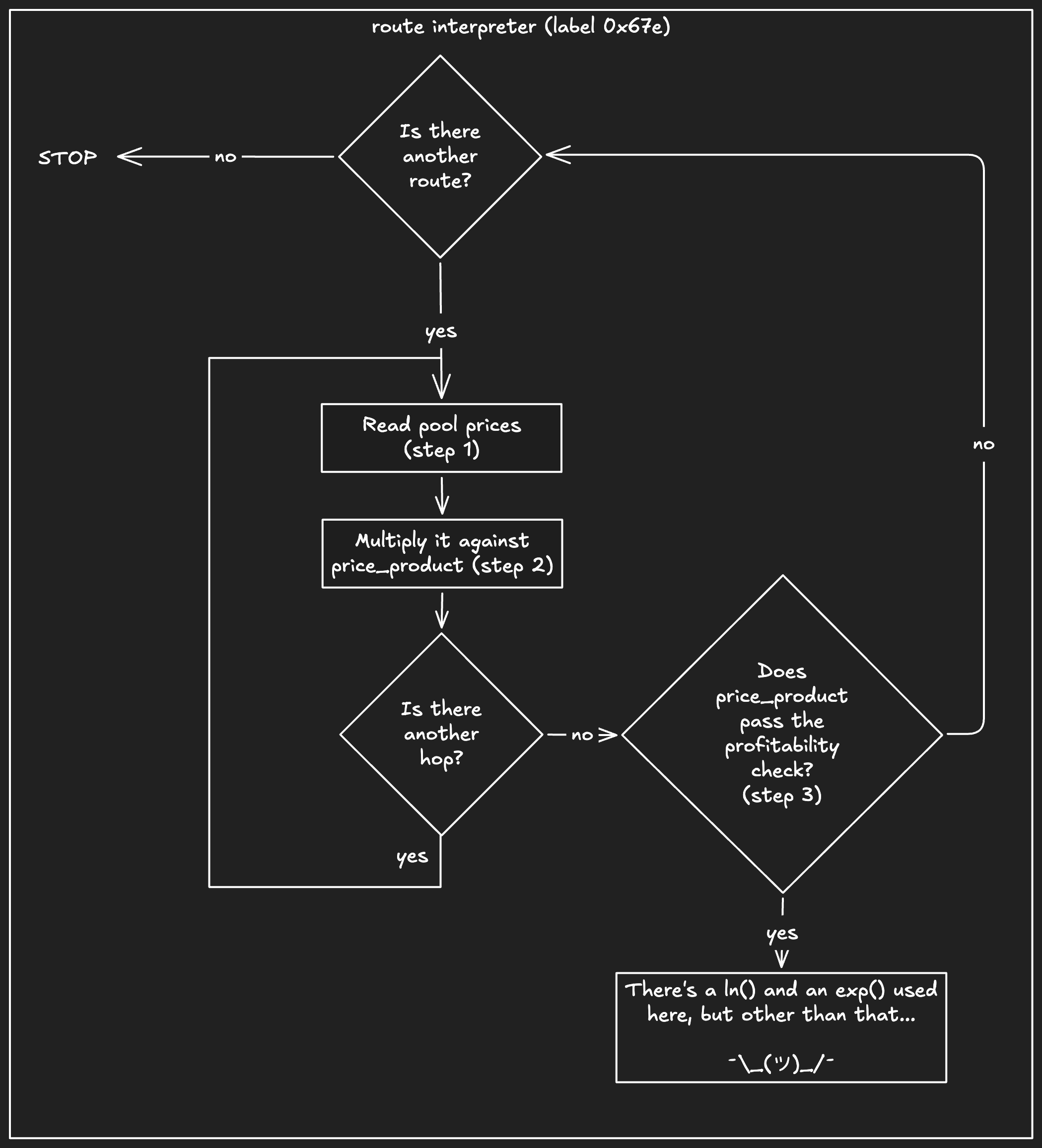
In this part we’ll uncover what’s inside that box at the lower right corner. You’ll see why these two functions are so critical that the contract and the whole strategy could’ve never been written without them.
Why does a bot that counts gas in single digits carry a hand-rolled math library instead of just multiplying numbers together? Because of the same reason humans invented logarithms four hundred years ago.
Logarithms turn multiplication into addition. In log space, a product becomes a sum and a huge multiplicative range becomes a modest additive one. Numbers that would overflow or shed precision when multiplied directly become small, well-behaved sums instead.
But if you visit log-land, you need a way to come back, and that’s what exp() is there for. That is why both constants are in the bytecode, they are the two ends of a tunnel.
Let’s go through it.
Why does it need these functions?
The EVM has no logarithm opcode and no floating point, and Solidity ships no standard library to paper over it. Well, to be honest, the EVM does have one exponentiation opcode, EXP, which raises integers to whole-number powers, but that’s a different animal from e^x for a fractional x, and there is no logarithm opcode at all.
Off-the-shelf fixed-point libraries (PRBMath, ABDK) would have covered it, and the operator passed on every one of them and built both functions by hand, in integer arithmetic, cheap enough to run in the hot path as described in the previous section.
What we haven’t found out yet is why, so let’s follow those two functions to the one place they get used, and let the code tell the story.
Every call to ln() and exp() in the contract lives inside a single routine that fires right after a route clears the profitability check gate. I am going to show you the whole thing before explaining any of it, the way I first met it, because the pieces do not make sense on their own. Hold on to the confusion, it is the point of this part of the exercise. It starts like this:
// what runs right after a route clears the profitability check gate.

// log of the `seed`, where that value comes from is shown just below
int256 lnSeed = ln(seed);

// log of 1.1x the bot’s token0 balance
int256 lnBalance = ln(balance * 11 / 10);
Again, this code was prettified from decompiled noise. Remember that the ln() function was inlined, so in reality it was far less readable, but it still worked like this. Right after deciding this route was revenue-positive, the first thing the contract does is take the logarithms of two numbers.
What I named seed is a curious value: it is not a single hardcoded constant, and it is not an argument passed into the function either. Instead it is picked from a handful of baked-in values by a nested if/else on token0, like this:
address token0 = pool.token0();

uint256 seed;
if (token0 == WETH) {
    seed = 1e13;
} else {
    // for any non-WETH token0, branch on its decimals
    uint8 decimals = token0.decimals();
    if      (decimals == 6)  seed = 10000;   // e.g. USDC, USDT
    else if (decimals == 8)  seed = 10;      // e.g. WBTC
    else if (decimals == 18) seed = 1e10;    // most 18-decimal ERC-20s
    else                     seed = 0;       // unrecognized decimals: a sentinel that aborts sizing
}
The contract takes the logarithm of a value, and that value depends entirely on what it treats as token0, and specifically on that token’s decimals.
Then, the second number it calculates the logarithm of, is 1.1 times the balance of the contract for that particular token0.
Continuing the execution, holding those two logarithms in hand, the code places two more points between lnSeed and lnBalance, each one a blend of the two weighted by a constant I will call W for now, and then feeds each point through exp() into a function we have not opened yet:
int256 lnSeed = ln(seed);
int256 lnBalance = ln(balance * 11 / 10);

// What I'm calling W is the constant 0x0893B2A3668E2500
// which is hardcoded both in decompiled code and opcodes view

// a and b land somewhere between lnSeed and lnBalance, positioned by W
int256 a = lnBalance - (lnBalance - lnSeed) * W / 1e18;
int256 b = lnSeed    + (lnBalance - lnSeed) * W / 1e18;

uint256 fa = mysteryFunction(exp(a));
uint256 fb = mysteryFunction(exp(b));
While the intent is hidden, the mechanics are not that complex: the code pins a range between two values and picks two points inside it, positioned by a constant. And then comes the strangest part. The contract enters a loop and runs the same little dance for a while. I renamed the moving ends lo and hi, they start out as lnSeed and lnBalance:
for (uint256 i = 0; i < 19; i++) {                 // at most 19 rounds, hardcoded into the bytecode
    if (gasUsedSoFar() > 4_000_000) break;         // spent too much gas: quit
    if (hi - lo < 2) break;                        // the ends nearly touch: quit

    if (fa > fb) {                                 // pull the top end in
        hi = b; b = a; fb = fa;
        a = hi - (hi - lo) * W / 1e18;
        fa = mysteryFunction(exp(a));              // exactly ONE new call per round
    } else {                                       // pull the bottom end in
        lo = a; a = b; fa = fb;
        b = lo + (hi - lo) * W / 1e18;
        fb = mysteryFunction(exp(b));              // exactly ONE new call per round
    }
}
Mechanically: each round compares the two measurements it holds, fa and fb, pulls one end of the range inward depending on which was bigger, recycles the stronger point with that odd little shuffle of b = a or a = b, and plants exactly one new point, placed by that same constant W, paying one more call to mysteryFunction(). The range shrinks every round, and the loop gives up after nineteen rounds, or after four million gas, or when the two ends all but touch.
So this is the ritual in full. Take the logarithms of two oddly chosen numbers and plant two points between them, positioned by a constant whose meaning we still don’t know. Feed each through exp() into a function we haven’t looked into yet. Then, again and again, chop off a slice of the range and plant one new point. We’re now juggling three unknowns:
- What is the
W = 0x0893B2A3668E2500constant? - What is the purpose of
mysteryFunction()? - Why are logarithms needed at all?
You can stare at the disassembly for a long time without cracking all three at once. The way in is to put the code down entirely and go think about the operator’s actual business for a few minutes. It will feel like we have dropped the thread but trust me, we haven’t.
A small detour: the hardest question in arbitrage
Forget the contract for a moment, and pretend you are the one running the operation. Your scanner has just found a real gap, the same asset is cheap in one pool and more expensive in another, and a round trip through them comes back with more than it left with. Everything in this series so far, the probes, the calldata menu, the profitability gate, has been about answering where the profit is and whether it is there. Here is the question none of it has asked: how much do you trade?
And no, the answer is not “as much as possible.” Every AMM pool moves against you as you trade into it. Buy a little WETH and the price barely budges. Buy a lot and you push the price up as you go, so each additional unit costs more than the last. Trade too small and you leave most of the opportunity on the table. Trade too large and you move the pools so far that you erase your own edge, sometimes turning a profit into a loss. Somewhere in between is a single best size, the peak of a hump-shaped profit curve.
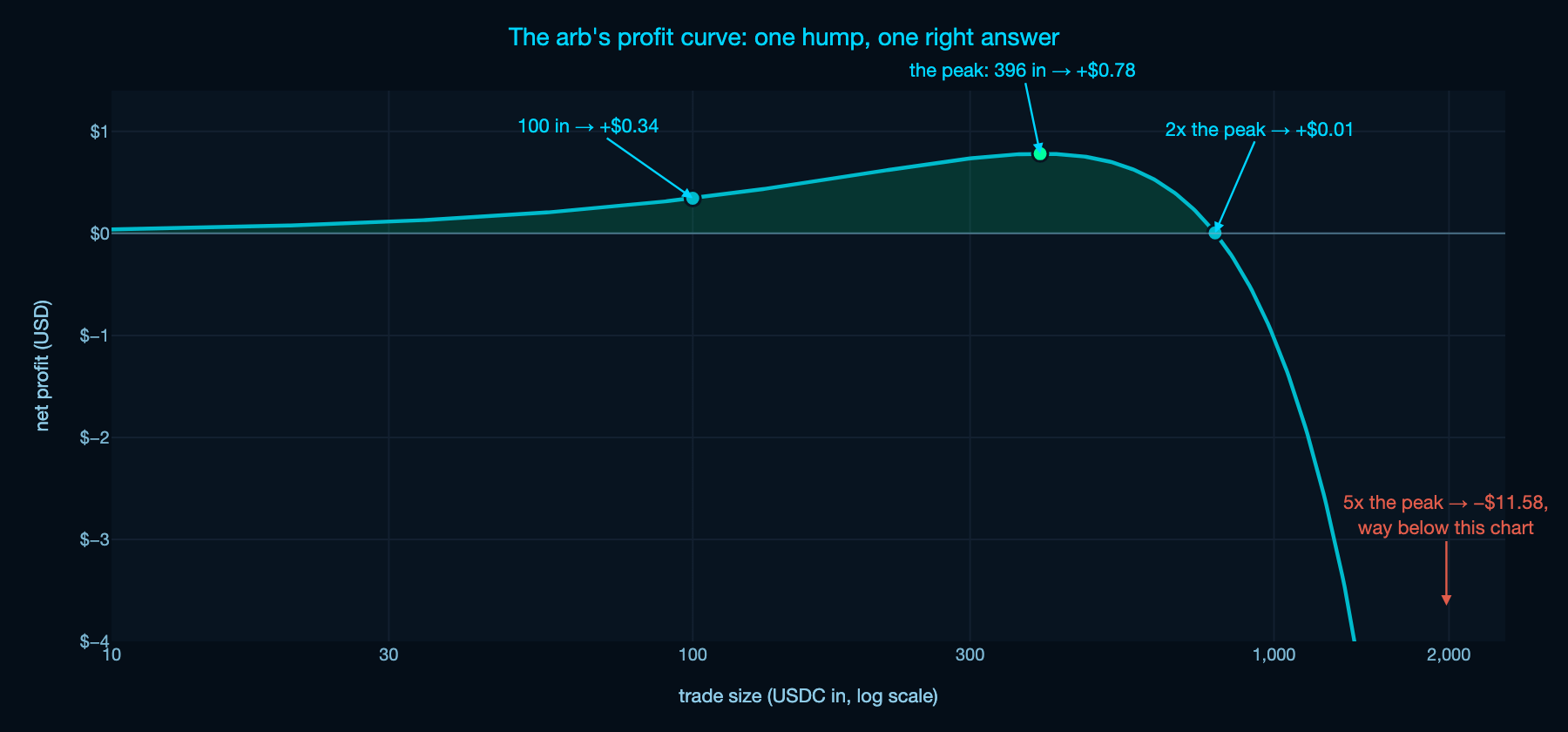
Take a toy version of the problem: two V2 pools holding the same WETH/USDC pair, one pricing WETH at 4,000 USDC and the other at 4,040, a fat one-percent gap, both charging the standard 0.3% fee.
- Push 100 USDC around that loop and you pocket about 34 cents.
- The best possible size turns out to be 396 USDC, which returns 78 cents.
- Push 792 USDC, merely double the optimum, and the profit collapses to a single cent.
- Push five times the optimum and the round trip loses eleven dollars.
The entire game lives inside less than one doubling of trade size: undershoot and you leave half the edge on the table, overshoot by 2x and you worked for free, overshoot further and you are paying the pools for the privilege. Sizing is not a refinement bolted onto finding the arb. Sizing is the arb.
The toy example, computed exactly, on the same log-scale view of trade sizes the contract itself uses. The shaded part is the entire profitable window. The curve tops out at 396 USDC in, is back to breakeven by roughly twice that, and dives so hard past it that the 5x point sits well over a full chart-height below the bottom edge.Sizing matters enormously, then. Fine, big deal, the obvious move is just solve for the peak, right?
You literally could, for the toy example above. Two constant-product pools compose into algebra simple enough that the optimal input has a closed form, differentiate the profit expression, set it to zero, and the best size falls out in one line. If every hop in every route were a V2 jar, sizing would be deterministic, a formula evaluated once, O(1).
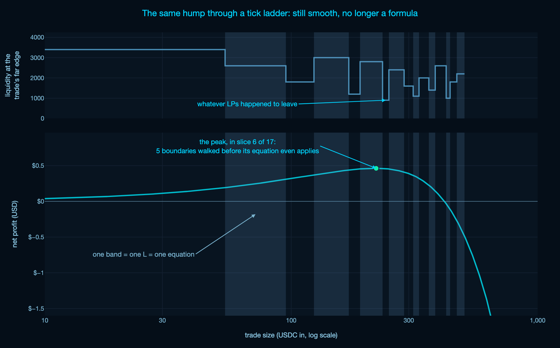
What kills this approach is concentrated liquidity. In a V3, Algebra, or V4 pool the liquidity your trade meets is a step function of price, defined by whatever ladder of ticks LPs happen to have built at that instant. The profit curve is still a single smooth-looking hump, but its equation changes every time the trade crosses a tick, so there is no one expression to differentiate.
The curve does not exist as math, it exists as data, and the only way to learn its height at a given size is to walk the whole trade through live pool state and see what comes out the other end. You are not doing that walk on paper either. Each one costs real gas.
The same toy route with the buy-side pool swapped for a concentrated-liquidity one, walked with the real tick-crossing math over a made-up but realistic ladder. Top: the liquidity the trade’s far edge is standing in, a staircase of whatever LPs left there. Bottom: the profit curve it produces.Notice the curve in the above chart stays perfectly smooth, that is the trap, it looks exactly as solvable as the V2 one. But every shaded band is a different equation with a different L plugged in, every band boundary below is a step above, and the boundaries move whenever LPs do. The peak happens to land in slice 6 of 17, something you can only discover by walking the five slices before it.
So here is the problem in its final form. You need to find the peak of a curve that rises, tops out, and falls: one hump, no second bump to fool you. And yes, you just saw that curve, but the picture is a luxury the contract can never have.
To draw it, my laptop walked the route hundreds of times, at leisure, for free. On-chain, computing one point of the curve and “seeing” that point are the same operation at the same price. There is no panoramic view. The curve is not invisible, it is priced per point, one full simulation per look.
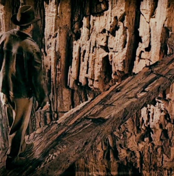
Remember the bridge scene in Indiana Jones and the Last Crusade, where Indy crosses an invisible chasm by throwing dirt ahead to reveal the walkway? This is that, with a pricing model.
A V2 route hands you the blueprint of the whole bridge: one formula, you compute where to stand, no dirt required. A concentrated route has no blueprint. The bridge is real, and it holds perfectly still while you cross, the pool state is frozen inside your transaction, but it is welded together from segments and no single drawing covers the span.
You’re going to need a lot more dirt.The only way to learn what is under the next step is to throw a handful of dirt and look, and every handful is one touch of the curve, one paid simulation. Then it gets worse one level up, because LPs rebuild the bridge between crossings, block by block, so the dirt you threw for the last opportunity tells you nothing about this one. You are still running a race vs gas and time, so how do you find the peak of the curve in as few touches as possible?
For those who actually remember their calculus class and are thinking “just find where the slope is zero”, let me tell you that won’t work here: there is no formula to differentiate, and even estimating a slope from samples costs two extra touches per estimate. What survives is an older and humbler idea called bracketing.
Touch the curve at two points in the middle of your range and compare them. With a single hump, the peak can never sit on the far side of the losing point, the curve out there can only keep falling. So everything beyond the loser is dead ground, so chop it off and repeat on the smaller range. No derivatives, no formulas, just comparisons, and the peak has nowhere to hide.
Done naively, that costs two fresh touches every round, one per interior point. This is the ternary search some of you will remember from a CS course. But in 1953 the mathematician Jack Kiefer noticed something interesting: place the two interior points at exactly the right depth, and after the chop, the surviving point lands precisely where the next round needs one of its two points to be.
One measurement gets recycled every round, so each round pays for a single fresh touch instead of two. Half the samples, same shrinkage. The catch is that the recycling only works for one placement. The shrunken bracket must be a scaled copy of the original with the survivor sitting where an interior point belongs, and it collapses into a small quadratic, r² = 1 − r, with a single positive root: the points must sit 61.8% of the way in from each end. Not roughly. Exactly
0.6180339887...Ring any bells?It looks suspiciously similar to the golden ratio,
1.6180339887..., and that’s no coincidence. The golden ratio is the number defined by the equation x² − x − 1 = 0, which has two roots: the celebrity,1.6180339887..., and a quieter sibling,−0.6180339887....Drop the minus sign and you have the golden ratio’s conjugate, the exact number Kiefer’s placement rule just produced (same beast from another angle: subtract one from the golden ratio, or divide one by it, and both give you
0.618..., the same digits all the way down.)The method is called golden-section search. Any search that recycles one point per round runs on this exact constant or it does not run at all.
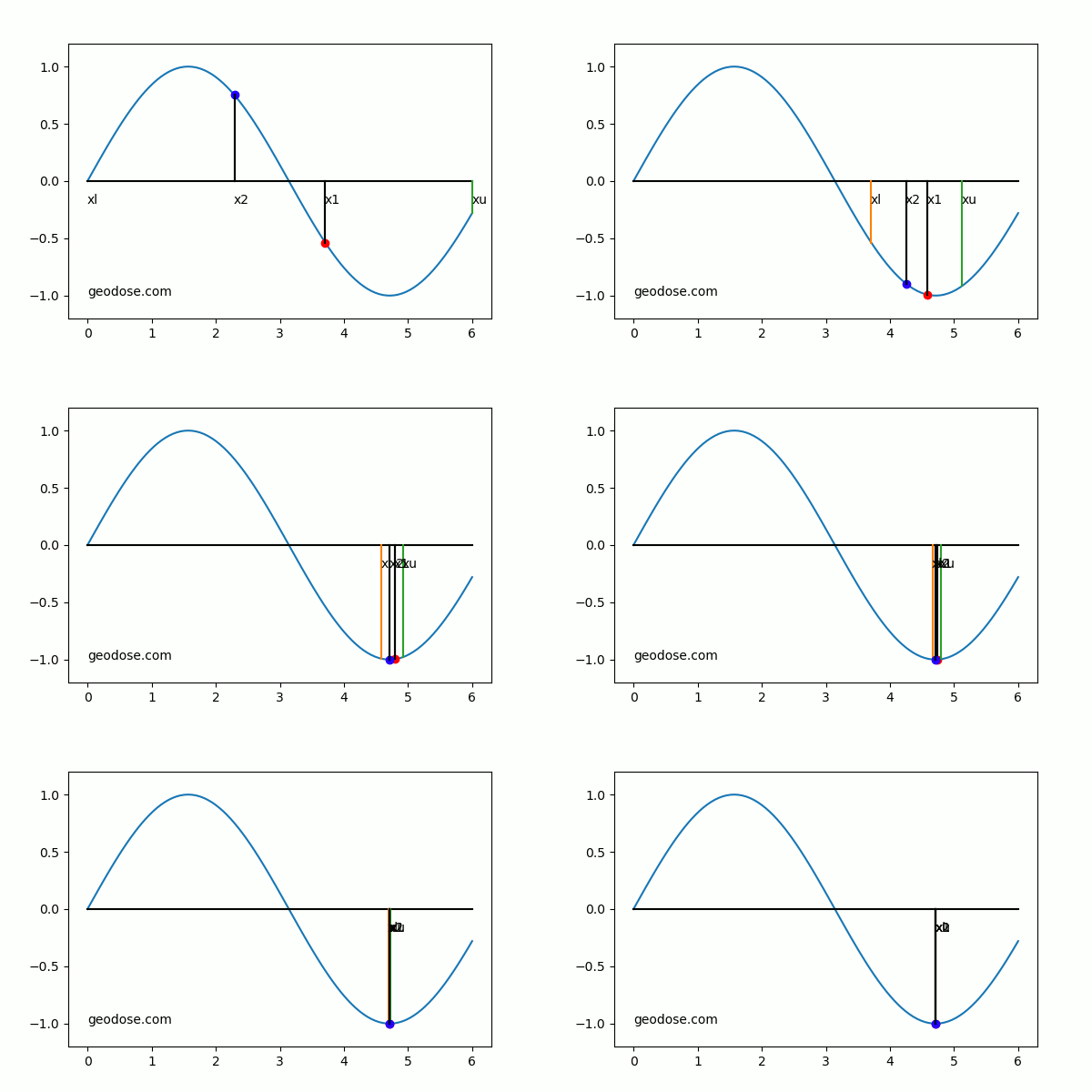
One peak, expensive samples, a tight budget. Golden-section search was invented for precisely this situation, and it looks like this in motion:
Golden-section search narrowing in on an optimum, one recycled sample per round, shown here hunting a minimum rather than a maximum (the two are identical up to a sign). Animation by Mlk80 (geodose.com), licensed under CC BY-SA 4.0.I know we said we need to search for peaks, but this gif was just too good not to use. You can clearly see how the bracket spans the whole curve at first (orange line on the left, green on the right), with the two test points dropped in the middle, and then, as the search closes in on the valley, either the upper or the lower bound collapses onto its nearest test point, which becomes the new boundary, leaving only a single fresh point to place inside the shrunken range.

End of detour. Now walk back to the disassembly with all this knowledge.
The number that gave it away
Two of the unknowns we mentioned a couple of lines above we can solve right here:
- A constant
W = 0x0893B2A3668E2500 - A
mysteryFunction()that was called two times, withexp(lnSeed)andexp(lnBalance)
The answer to the third one, about why any of this happens in log land, becomes obvious after that. Let’s start with the constant, pulling W out of the bytecode and dividing by 1e18 (the same move we have used on every constant in this article)
There it is. The golden ratio’s conjugate, to ten decimal places, hardcoded in the bytecode of the contract. You just don’t land on that number by accident.
That’s the ritual we could not read, a golden-section search.
This section of the arb workflow in the contract is looking for the peak of its own profit curve, live, on-chain, inside the very transaction that found the arb. And the moment you see that, the other unknowns fall in quick succession, because a golden-section search needs the props we could not explain.
The two oddly chosen numbers are the bracket, the search’s opening claim that “the best trade size lies somewhere in here”. The seed is the floor, the smallest trade worth even thinking about:
- 1e13 wei is about two cents of ether
- 10000 units of a 6-decimal stablecoin is a cent
- 10 units of an 8-decimal token is roughly a cent of WBTC
Three decimal dialects which share a similar floor (the generic 18-decimal fallback sits far lower, sensibly so, since a random 18-decimal token’s unit price could be anything). And balance * 11 / 10 is the ceiling, a touch more than everything the bot could deploy. The answer sits between dust and all-we-have.
mysteryFunction() is the touch. The thing every candidate gets fed into, and its outputs are what the loop compares, so it can only be the height measurement: it takes a real token amount, pushes it around the entire circular route against live pool state, and reports how much comes out the other end. It is a simulator, so from here on I will call it simulate(). It also happens to be the heaviest thing the contract ever runs, and we will open it up before this section is over. And the loop is Kiefer’s dance, step for step. I’ve used proper names now, so let’s re-read it with fresh eyes.
int256 lnSeed = ln(seed);
int256 lnBalance = ln(balance * 11 / 10);

// the bracket ends
int256 lo = lnSeed;
int256 hi = lnBalance;

// the two interior points, placed inside the bracket by W
int256 a = hi - (hi - lo) * W / 1e18;
int256 b = lo + (hi - lo) * W / 1e18;

// the probes
uint256 fa = simulate(exp(a));
uint256 fb = simulate(exp(b));

for (uint256 i = 0; i < 19; i++) {                 // at most 19 rounds, hardcoded into the bytecode
    if (gasUsedSoFar() > 4_000_000) break;         // spent too much gas: quit
    if (hi - lo < 2) break;                        // the ends nearly touch: quit

    if (fa > fb) {                                 // pull the top end in
        hi = b; b = a; fb = fa;
        a = hi - (hi - lo) * W / 1e18;
        fa = simulate(exp(a));                     // exactly ONE new call per round
    } else {                                       // pull the bottom end in
        lo = a; a = b; fa = fb;
        b = lo + (hi - lo) * W / 1e18;
        fb = simulate(exp(b));                     // exactly ONE new call per round
    }
}
fa > fb asks which candidate made more money, the end that gets pulled in is the dead ground where the peak cannot be, the shuffle of b = a or a = b is the recycled measurement, and each round pays for exactly one fresh simulation, which is the entire reason 0.618 is in the code at all. The number is forced by the algebra of recycling one sample per round. Even the exit tests now read as part of the design: hi - lo < 2 is the bracket collapsing to nothing, and the gas check deserves its own moment, which it will get shortly.
This is what the operator needed ln() and exp() for. The search runs entirely in log space: its two ends are lnSeed and lnBalance, every point it tries between them is a logarithm, and exp() is the escape hatch, called only when a candidate has to leave log space and become a real token amount for the simulator. ln() is the door in, exp() is the door back out of every step. The two functions we’ve been looking at were the entrance and the exit.
Why the search lives in log-land
Which begs the question: why dig that tunnel in the first place?
Running the search in log space is not just a geek flex, it’s the most intelligent decision for this particular environment. It’s all about making numerical methods survive on hostile hardware. There are a few layers to this.
int256 lnSeed = ln(seed);   // seed is 1e13 for WETH
int256 lnBalance = ln(balance * 11 / 10);
-
The first layer is the shape of the search space. Look at where the bracket’s two ends come from. The
seedfor a WETH route is 1e13 wei, about two cents worth of ether, the smallest trade even worth thinking about. The other end is the bot’s entire balance plus ten percent. Those two ends can easily sit five orders of magnitude apart. Now imagine running the search on raw token amounts. A golden-section bracket places its first two probes at 38% and 62% of the way across, and on a bracket from 1e13 to 1e17 both of those land within a factor of three of the top. The entire bottom of the range, every modest-sized opportunity, would go unsampled until the loop had nearly exhausted its iteration budget narrowing its way down. In log space every step is multiplicative instead of additive. The probes split the range by orders of magnitude, and a sweet spot near $5 gets found exactly as fast as one near $50,000. -
The second layer is what “precision” even means here. A linear bracket converges to an absolute width, and an absolute target is the wrong kind of target when you do not know the answer’s scale in advance: narrowing to within a few wei is meaningless slack when the best size is near 1e17 and wasted effort when it is near 1e13. A log bracket converges to a relative width, the answer pinned to within a multiplicative factor, which is the same quality of answer at every scale. It also explains the loop’s otherwise absurd-looking exit test,
hi - lo < 2. Those are fixed-point log units, so the test does not mean “within two wei”, it means “the two ends differ by a vanishingly small ratio”, a relative-error test wearing an integer costume. -
The third layer is the one the EVM forces. Look again at how the interior points are built: each one is a weighted blend of the two ends. Blend in log space, exponentiate, and what you have computed in linear terms is a weighted geometric mean, lo^0.382 · hi^0.618. To compute that directly on token amounts you would need to raise numbers to fractional powers, and the EVM has no opcode for that. The standard trick for faking x^0.618 is, precisely, exp(0.618 · ln(x)). You end up needing
ln()andexp()either way. So the operator put the entire search on the log side of the tunnel, where every blend is two multiplications and a subtraction, pays theexp()toll only when a candidate has to become a real token amount for the simulator, and as a bonus every number the loop’s arithmetic touches stays in a narrow, overflow-proof band while the raw amounts themselves sprawl across half of uint256’s range. The tunnel was never optional. The search could not have been written any other way.
The bill for the calculus
There is one piece of restraint left to admire, the loop runs simultaneously on a clock and a budget.
It takes at most nineteen iterations, no matter what, and before every simulation it checks how much gas it has already burned, stopping the instant that figure crosses four million and taking the best size found so far. That is an optimizer whose termination condition includes the cost of running the optimizer. It will not chase the mathematically perfect trade size if the chase would eat the profit it is trying to capture. For an article series about a bot that counts gas in single digits, nothing captures the philosophy better than an algorithm that watches its own gas gauge and knows when to quit.
for (uint256 i = 0; i < 19; i++) {                 // at most 19 rounds, hardcoded into the bytecode
    if (gasUsedSoFar() > 4_000_000) break;         // spent too much gas: quit
    if (hi - lo < 2) break;                        // the ends nearly touch: quit

    if (fa > fb) {                                 // pull the top end in
        hi = b; b = a; fb = fa;
        a = hi - (hi - lo) * W / 1e18;
        fa = simulate(exp(a));                     // exactly ONE new call per round
    } else {                                       // pull the bottom end in
        lo = a; a = b; fa = fb;
        b = lo + (hi - lo) * W / 1e18;
        fb = simulate(exp(b));                     // exactly ONE new call per round
    }
}
Observant readers might be wondering about the two magic numbers wrapped around that loop, and it turns out neither is arbitrary. Both sit hardcoded in the bytecode: a PUSH1 0x13 (19) capping the round counter, and a PUSH3 0x3d0900 (4,000,000) compared against a reading of the GAS opcode before every fresh simulation.
The gas figure is a budget. The 19, though, is mathematics. Let’s count the samples: two simulations seed the bracket and every pass of the loop adds exactly one more, so a full run tastes the curve at most 21 times. Each pass multiplies the bracket’s width by 0.618, so nineteen passes shrink it to about one ten-thousandth of where it started. Because the bracket lives in log space that is relative precision: even with the two ends five orders of magnitude apart, the answer comes out pinned to roughly a tenth of a percent of the optimal size.
That is the textbook golden-section bargain, sample count growing only with the logarithm of the precision you demand. And for this job, a tenth of a percent is the same as exact, because the profit curve is flat at its very top, that is what being a peak means, so missing the optimum by 0.1% in size costs on the order of a millionth of the profit. A twentieth round would spend an entire tick-walking simulation to buy precision worth less than dust. Nineteen is exactly the point where the golden ratio’s shrinkage stops paying for its own samples.
Gas is where it gets concrete. I went back over every scan window of this operation for which we have both gas and revenue data, covering this contract plus the operator’s subsequent iterations, 761 profitable executions in all, and compared each winning transaction against the median losing probe with the same calldata shape.
A losing probe of the common three-hop shape burns about 43k gas. The median winning transaction burns about 459k. So everything behind the gate, the pool snapshot, the golden-section search, and the real execution it feeds, costs a median of roughly 410k extra gas, which at Arbitrum’s ~0.02 gwei worked out to about two cents per win (median $0.019, mean $0.024), and that median barely moves from one deployment to the next.
Splitting that number cleanly between the search and the execution would take a full instruction trace of a winning transaction, but the shape of the work says the search dominates: up to 21 read-only rehearsals of the route versus one paid performance, and the loop’s own bailout reserves a 4M gas budget for the rehearsals alone.
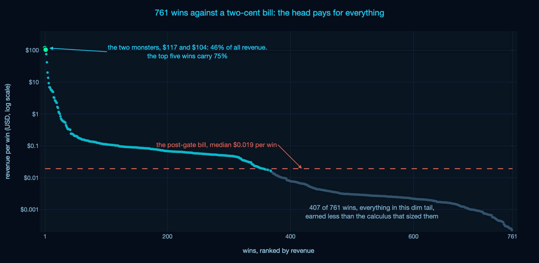
Every profitable execution in the dataset, ranked by revenue, against the post-gate bill. Each dot is compared with its own transaction’s bill, not just the dashed median, and the dots dim at the exact point where the trade stopped paying for its own sizing. Mind the log scale: the head’s dominance is far more brutal than it looks, the gap between the monsters and the median win is four orders of magnitude.
Is two cents a lot? Across those 761 wins it adds up to about eighteen dollars, roughly 4% of the $481 the operation grossed in the same windows. As an aggregate tax on profits, small. The distribution underneath that average is the revealing part, though: the median win returned about one cent, so for 407 of the 761 winners, more than half, the post-gate machinery cost more than the trade it sized brought back, while the two largest wins ($117 and $104) hauled in 46% of the entire revenue by themselves, and the top five carried three quarters of it.
The optimizer is not there to make the median trade profitable, and it demonstrably does not. It is there so that when the fat opportunity finally surfaces, the size is right, and two cents of calculus on a hundred-dollar trade is as close to free as anything gets on-chain.
The last thing to explain is the cost of a single sample, and it is where the last unopened function finally matters.
The last function: the simulator
The simulate() function is the heaviest thing the contract owns and the last one we have not opened. Its job is narrow to describe and enormous to execute: given one candidate trade size, push that amount all the way around the circular route and report what comes back. One number in, one number out. Everything between is where the gas goes.
What one taste actually costs
The reason a single probe is expensive is that a route is not one pool, it is a chain of them, and each link is a different machine. The simulator walks the hops in order, feeding each pool’s output into the next, and at every hop it has to speak whatever pricing dialect that pool was built in. Stripped of the fixed-point bookkeeping and the decompiler’s noise, the shape is this:
// simulate(amount, route): push `amount` around the whole loop, return the output.
function simulate(uint256 amount, Route route) internal returns (uint256) {

    // Hops are walked in route order, or in reverse, chosen by the `direction` flag.
    for (each hop in route) {
        if (amount == 0) break;              // nothing left to trade

        Pool pool = decrypt(hop.pool);       // address stored XOR-masked, unmasked here
        bool zeroForOne = directionFor(hop);

        if (pool.kind == V2) {
            // A jar of two reserves: one closed-form step, using this pool’s own fee.
            amount = constantProductOut(amount, pool, zeroForOne);
        } else {
            // Concentrated liquidity (V3 / Algebra / V4): no formula, a walk.
            (uint160 sqrtP, int24 tick, uint128 L) = (pool.sqrtPriceX96, pool.tick, pool.liquidity);
            uint256 out = 0;

            while (amount > 0) {
                if (gasSpentInThisWalk() > 1_000_000) {
                    amount = 0; break;  // per-taste fuse
                }
                if (sqrtP <= MIN_SQRT || sqrtP >= MAX_SQRT) {
                    amount = 0;
                    break;
                }
                int24 next = nextInitializedTick(pool, tick, zeroForOne); // a lookup
                uint160 sqrtNext = getSqrtRatioAtTick(next);   // Uniswap’s math
                (uint256 used, uint256 got) = computeSwapStep(sqrtP, sqrtNext, L, amount, pool.fee);

                amount -= used;
                out += got;
                if (crossedInto(next)) {
                    L = applyNet(L, liquidityNet(pool, next), zeroForOne);
                }
                (sqrtP, tick) = (sqrtNext, next);
            }
            amount = out;
        }
    }
    return amount;
}
The V2 branch is the whole reason the word jar fit back in the price-reading section: two reserves, one algebraic step, done. The else branch is where the cost lives. A concentrated-liquidity pool keeps its money in slices along the price line, so the walk crawls the price from one tick boundary to the next, and at every boundary it must do three expensive things: look up where the next slice of liquidity begins, convert that tick into a price with Uniswap’s exact bit-twiddling routine, and read how much liquidity is added or removed at the crossing.
A route with two concentrated hops can cross a dozen ticks, and every crossing is external calls and heavy arithmetic. That is one point on the profit curve. The golden-section search asks for up to twenty-one of them.
Three dialects, and a duck-typing fallback
The three concentrated families store the same facts in three incompatible ways, and simulate() speaks all of them. What is clever is how it tells them apart, because it is the same trick twice.
For V3 and Algebra, the bot does not carry a flag saying which is which. It just tries the Uniswap getter and, if the call reverts, retries with Algebra’s name for the identical data. The tick bitmap is read as tickBitmap(word). On failure it falls back to tickTable(word). The price snapshot is read as slot0(). On failure, globalState(). It literally speaks Uniswap first and switches to Algebra’s accent only when Uniswap’s word is not understood. Pretty much runtime duck-typing, in hand-rolled EVM.
For V4 there is no getter to try, because V4 has no per-pool contract at all, the same fact we met when reading prices. Every pool lives as raw storage inside the one PoolManager, so the simulator computes the storage slot itself and reads it with extsload. The tell is in the constants: it hashes the pool id against slot 6, then offsets by 5 to reach the tick bitmap and 4 to reach a tick’s data. Those three numbers, 6, 5, 4, are not arbitrary, they are POOLS_SLOT, TICK_BITMAP_OFFSET, and TICKS_OFFSET straight out of Uniswap’s own StateLibrary. The bot is not just reading V4 storage, it is reading it with Uniswap’s own floor plan memorized.
The fingerprints: Uniswap’s own constants
We’ve been circling around this fact for a while: the operator rebuilt Uniswap’s swap math inside their own contract, and left the fingerprints to prove it. Uniswap ships an on-chain Quoter whose entire job is to answer “if I traded this much, what would I get.” This bot ignores it and reimplements the whole tick-walking simulation locally, and the reused code is not paraphrased, it is copied constant for constant.
The clearest fingerprint is the tick-to-price conversion, getSqrtRatioAtTick(). Uniswap computes it without ever calling pow(), by folding in one precomputed factor for each set bit of the tick. The bot’s version folds in the same nineteen magic numbers, in the same order:
// getSqrtRatioAtTick, rebuilt bit for bit. One precomputed factor per set bit.
if (tick & 0x1)     ratio = (ratio * 0xfff97272373d413259a46990580e213a) >> 128;
if (tick & 0x2)     ratio = (ratio * 0xfff2e50f5f656932ef12357cf3c7fdcc) >> 128;
if (tick & 0x4)     ratio = (ratio * 0xffe5caca7e10e4e61c3624eaa0941cd0) >> 128;
if (tick & 0x8)     ratio = (ratio * 0xffcb9843d60f6159c9db58835c926644) >> 128;

// ... fifteen more lines, one per bit ...
if (tick & 0x40000) ratio = (ratio * 0x48a170391f7dc42444e8fa2)         >> 128;
These are byte-for-byte the constants in Uniswap V3’s TickMath. The bounds the walk checks against, 0x01000276a4 and 0xfffd8963efd1fc6a506488495d951d5263988d25, are MIN_SQRT_RATIO + 1 and MAX_SQRT_RATIO from the same file. And the 512-bit multiply-and-divide that the swap step leans on is Uniswap’s FullMath.mulDiv, recognizable by the little Newton-Raphson modular inverse it seeds with 3 · denominator XOR 2, inlined right there in the bytecode. Three separate Uniswap libraries, transplanted whole.
Why carry all that, instead of calling the Quoter?
Gas and control, which btw is also a factor on the choice of hand-rolling the ln() and exp() functions instead of linking a library.
The official Quoter is a separate contract, so every call to it is a cross-contract jump, and it is written for correctness and generality, not for being hammered twenty-one times inside a probe that has to stay cheap. Inlining the simulator keeps the entire search in one execution context with no per-sample call overhead. But the real prize is interruptibility.
Look again at the fuse inside the walk: before every tick step, the local simulator checks how much gas it has burned and, the instant it crosses a million, abandons the walk. And when it abandons, or when a lookup reverts, or when the price runs out of bounds, it does not throw. It sets the amount to zero and returns, so a hopeless candidate simply scores nothing and the search moves on to the next one.
That is the whole reason the math had to be rebuilt. A gas gauge welded to the inside of the swap loop, and a failure that costs a zero instead of a revert, are two things the official Quoter would never hand you. The heavy tick-walking simulator and the gas-aware search are one idea seen from two ends: the operator rebuilt Uniswap’s math precisely so they could bolt their own budget onto it.
It is the same instinct as the cheap no from the very first section, pushed all the way down into the most expensive code in the contract. Even when it spends, it refuses to overspend.
The hidden shape, revealed
The three threads we pulled turn out to be from the same rope, and the economic model from Part 1 has stopped being a mystery. Every probe transaction runs the same function. It reads a few spot prices, chains them into a product, and holds that product up against profitScale. About 999 out of 1000 times the product does not clear the bar, and the contract stops right there, having spent a fraction of a cent and touched nothing.
That is the flat expanse of reverts Part 1 charted. The rare time the product does clear, a second, far heavier machine kicks in behind the gate: the contract takes a full live snapshot of every pool, drops into log space with its hand-rolled ln(), and runs a gas-budgeted golden-section search that calls its hand-rolled exp() and its local swap simulator up to nineteen times to find the single best trade size, then hands that number off to be executed.
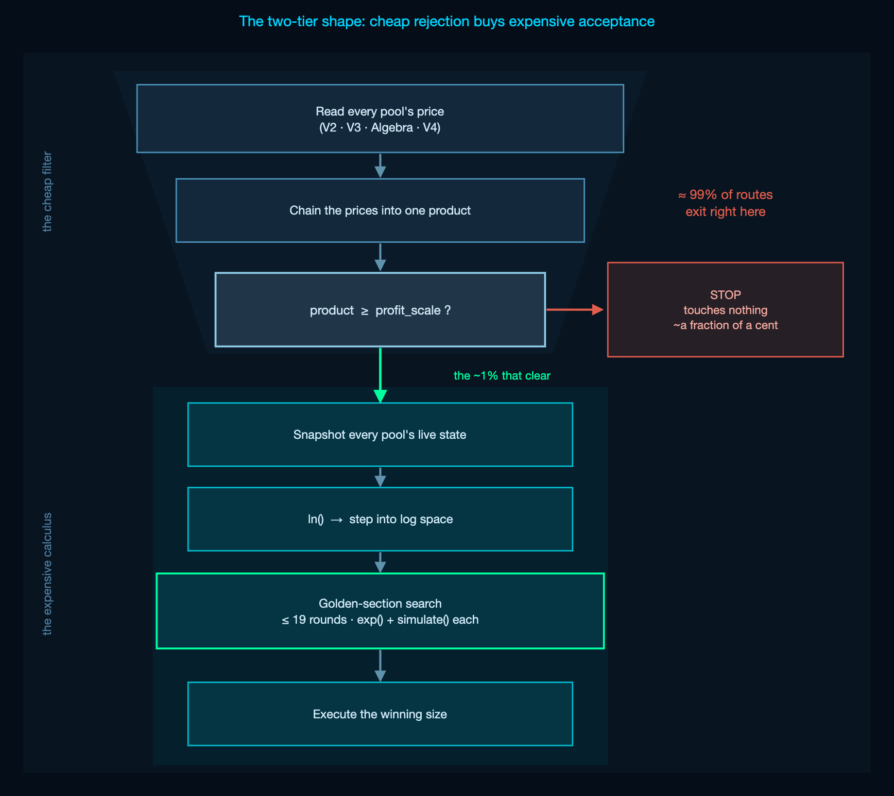
The whole of the main function every probe runs, in one picture. Everything above the gate is a few storage reads and one multiply, which is why the bot can afford to run it on thousands of routes that go nowhere. Everything below the gate, the live snapshot, the logarithms, the nineteen-step search each tasting the profit curve with exp() and the simulator, only ever runs on the rare route that clears the bar
That two-tier shape is the answer to the question Part 1 left open. The bot can afford to be almost always wrong because being wrong is nearly free: the gate is a few reads and a multiply.
And it can afford to be genuinely precise on the rare occasion it is right, spending real gas on logarithms and a nineteen-step search, because it has already spent almost nothing on the thousands of times it was wrong. Cheap rejection is what buys expensive acceptance. The filter and the calculus are not two separate bits of cleverness, they are the same design decision seen from two ends.
We met
profitScaleagainI promised in Part 2 that we would see
profitScaleagain, and we found it exactly where I said the trail had gone cold: standing guard at the gate, the operator’s dial for how much apparent edge to demand from cheap spot prices before paying for the expensive certainty of a full search.I still cannot hand you its precise units, and I would rather keep saying that than pretend otherwise. But it is no longer a number floating in a header with no home. It has a job, and it is an important one.
We finally opened the kitchen. The menu from Part 2 told the contract where to look. The math in here is how it decides, in a breath of gas, whether looking was worth it, and if so, exactly how hard to swing: a logarithm to get into the search, an exponential to get out of each step, a hundred-year-old optimizer that watches its own gas gauge, and a hand-built simulator to taste the profit curve one expensive point at a time.
It is the cleverest code in the contract, and there is something a little humbling about finding it inside a bot most people would dismiss as a dumb shotgun firing transactions at the wall.
There is only one thing left.
The search ends with a number: the optimal amount to trade. Everything up to now has been the contract deciding and computing, touching no assets, moving no tokens, risking nothing. The winning size gets packed up and handed to Uniswap V4’s flash-accounting machinery.
That is where the abstract finally becomes real money. It is where the rubber meets the road, and its design has to survive contact with pools it cannot always use, and blind spots it cannot always see.